Quote risk and revaluation for a mixed portfolio

A pay-fixed swap can offset some of a bond’s interest-rate exposure. To examine that offset, we combine a USD 1 million pay-fixed swap, a USD 500,000 fixed-rate bond at zero Z-spread and a USD 2 million caplet. The market is the illustrative SOFR curve and Black surface dated 24 February 2026.

We value the trades, aggregate sensitivities by input quote and compare their linear P&L estimate with full scenario revaluation:

\[\Delta V\approx\sum_j\frac{\partial V}{\partial q_j}\Delta q_j.\]

All position values are in USD. Rate, volatility and bond-spread inputs use their own quotation units. The calculation measures today’s portfolio risk; legal netting and future credit exposure are developed in the XVA study. Setup.

Computational study. Canonical notebook · Companion files and setup. Download this notebook.

This page renders saved outputs; the documentation build does not execute it. Run the canonical notebook from its own directory with the checkout-built binding to reproduce the computation. Each study records its market inputs and numerical assumptions.

import matplotlib.pyplot as plt
import pandas as pd
import quantsupport as qs
from market_data import load_market

market = load_market()
ref = market.quotes.reference_date
swap = qs.Swap(
    identifier="BOOK-SWAP",
    start_date=ref,
    maturity_date=ref + "5Y",
    notional=1_000_000,
    fixed_rate=0.04,
    currency=qs.Currency.USD,
    market_index=qs.MarketIndex.SOFR,
)
bond = qs.FixedRateBond(
    identifier="BOOK-BOND",
    start_date=ref,
    maturity_date=ref + "5Y",
    notional=500_000,
    rate=0.045,
    currency=qs.Currency.USD,
    payment_frequency=qs.Frequency.Semiannual,
)
caplet = qs.CapletFloorlet(
    identifier="BOOK-CAPLET",
    fixing_date=ref + "2Y",
    start_accrual_date=ref + "2Y",
    end_accrual_date=ref + "2Y3M",
    payment_date=ref + "2Y3M",
    strike=0.045,
    currency=qs.Currency.USD,
    market_index=qs.MarketIndex.SOFR,
    payoff_type=qs.CapletFloorletType.Caplet,
)
portfolio = [
    qs.Trade(swap, ref, qs.Side.PayShort),
    qs.Trade(bond, ref, pricing_anchor=qs.BondPricingAnchor.z_spread(0.0)),
    qs.Trade(caplet, ref, notional=2_000_000),
]

Valuing the positions

Each trade receives requests supported by its pricer. The swap supplies its par coupon and cashflows, the bond adds yield and duration analytics, and the caplet supplies value and sensitivities. The bond’s zero Z-spread is an explicit trade anchor.

We retain trade identifiers when collecting the results. Grouping risk by pillar then adds signed exposure to the same market input across positions, so hedging offsets remain visible. Unavailable analytics stay unpopulated.

extra_requests = {
    swap.identifier: [qs.Request.FairRate(0), qs.Request.Cashflows],
    bond.identifier: [
        qs.Request.YieldToMaturity,
        qs.Request.ModifiedDuration,
        qs.Request.ZSpread,
        qs.Request.Cashflows,
    ],
    caplet.identifier: [],
}
results = []
risk_tables = []
cashflow_tables = []
context = qs.PricingContext(
    quotes=market.quotes,
    curves=market.curves,
    csa_policy=market.csa_policy,
    volatility_surfaces=market.volatility_surfaces,
)

with context:
    for trade in portfolio:
        result = context.evaluate(
            trade,
            [
                qs.Request.Value,
                qs.Request.Sensitivities,
                *extra_requests[trade.instrument.identifier],
            ],
        )
        results.append(
            {
                "trade": result.identifier,
                "pv_usd": result.price,
                "fair_rate": result.fair_rate,
                "ytm": result.yield_to_maturity,
                "modified_duration": result.modified_duration,
            }
        )
        risk_tables.append(result.sensitivities.assign(trade=result.identifier))
        if result.cashflows is not None:
            payments = result.cashflows.loc[
                result.cashflows["payment_date"] > str(ref)
            ].copy()
            payments["fixing"] = payments["fixing"].astype(float)
            payments["signed_amount_usd"] = payments["amount"]
            cashflow_tables.append(payments.assign(trade=result.identifier))

valuation = pd.DataFrame(results).set_index("trade")
trade_risk = pd.concat(risk_tables, ignore_index=True)
portfolio_risk = trade_risk.groupby("pillar")["value"].sum()
portfolio_pv = valuation["pv_usd"].sum()
print(f"Portfolio PV: USD {portfolio_pv:,.2f}")
valuation

Portfolio PV: USD 513,286.83

	pv_usd	fair_rate	ytm	modified_duration
trade
BOOK-SWAP	1664.991324	0.040368	NaN	NaN
BOOK-BOND	510478.041062	NaN	0.044142	3.786059
BOOK-CAPLET	1143.799136	NaN	NaN	NaN

Scaling the risk report

A sensitivity is the PV derivative per unit change in its named input. Multiply rate and Z-spread derivatives by 1e-4 for a one-basis-point move, and Black-volatility derivatives by 0.01 for one volatility point.

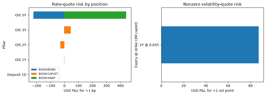
The construction specifications identify each quote family. The matrix below preserves individual trade contributions before adding their signed total, allowing us to inspect where the swap offsets the bond.

rate_labels = market.curves[0].to_dict()["quotes"]
vol_labels = market.volatility_surfaces[0].to_dict()["quotes"]

rate_derivatives = portfolio_risk.reindex(rate_labels, fill_value=0)
rate_risk = pd.DataFrame({"dPV_dQuote": rate_derivatives})
rate_risk["pnl_plus_1bp_usd"] = rate_derivatives * 1e-4
vol_derivatives = portfolio_risk.reindex(vol_labels, fill_value=0)
vol_risk = pd.DataFrame({"dPV_dQuote": vol_derivatives})
vol_risk["pnl_plus_1vol_point_usd"] = vol_derivatives * 0.01
spread_risk = portfolio_risk[portfolio_risk.index.str.endswith(".ZSpread")] * 1e-4

contributions = trade_risk.pivot_table(
    index="pillar", columns="trade", values="value", aggfunc="sum", fill_value=0
)
rate_contributions = contributions.reindex(rate_labels, fill_value=0) * 1e-4
rate_contributions["portfolio"] = rate_contributions.sum(axis=1)
rate_contributions

trade	BOOK-BOND	BOOK-CAPLET	BOOK-SWAP	portfolio
pillar
FixedRateDeposit_USD_SOFR_1D	-0.141782	-0.000318	0.277281	0.135181
OIS_USD_SOFR_1Y	-0.357122	-0.938500	0.305058	-0.990564
OIS_USD_SOFR_2Y	-0.351285	-28.670557	-0.133328	-29.155170
OIS_USD_SOFR_3Y	-1.273675	44.490311	0.676114	43.892750
OIS_USD_SOFR_5Y	-222.268675	0.000000	441.809500	219.540824
OIS_USD_SOFR_7Y	0.000000	0.000000	0.000000	0.000000
OIS_USD_SOFR_10Y	0.000000	0.000000	0.000000	0.000000
OIS_USD_SOFR_30Y	0.000000	0.000000	0.000000	0.000000

rate_plot = rate_contributions.drop(columns="portfolio")
rate_plot = rate_plot.loc[rate_plot.abs().max(axis=1) > 1e-8].copy()
rate_plot.index = rate_plot.index.str.replace(
    "FixedRateDeposit_USD_SOFR_", "Deposit ", regex=False
).str.replace("OIS_USD_SOFR_", "OIS ", regex=False)
vol_plot = vol_risk.loc[
    vol_risk["pnl_plus_1vol_point_usd"].abs() > 1e-8, "pnl_plus_1vol_point_usd"
]
vol_plot = vol_plot.nlargest(6).copy()
vol_plot.index = (
    vol_plot.index.str.replace("CapletFloorlet_USD_SOFR_3M_", "", regex=False)
    .str.replace("_Absolute_", " @ ", regex=False)
    .str.replace("_Straddle_Black", "", regex=False)
)

fig, axes = plt.subplots(1, 2, figsize=(11, 4))
rate_plot.plot.barh(stacked=True, ax=axes[0])
axes[0].set(
    title="Rate-quote risk by position", xlabel="USD P&L for +1 bp", ylabel="Pillar"
)
axes[0].legend(loc="lower left", fontsize=8)
vol_plot.plot.barh(ax=axes[1])
axes[1].set(
    title="Nonzero volatility-quote risk",
    xlabel="USD P&L for +1 vol point",
    ylabel="Expiry @ strike (3M caplet)",
)
plt.tight_layout()
plt.show()

Comparing derivatives with full revaluation

A small central bump checks the aggregate local derivative. We shift deposit and OIS rate quotes together, rebuild the market and reprice the portfolio, while retaining volatility quotes and the bond’s zero spread.

A central difference using ±1 bp should closely match the summed rate-quote derivatives. We also apply a +100 bp stress to examine the effect of curvature and recalibration on the linear prediction.

def portfolio_under_quote_shift(bump, labels=rate_labels):
    shocks = [
        qs.Shock(target=label, value=bump, shock_type=qs.ScenarioType.Absolute)
        for label in labels
    ]
    context = qs.PricingContext(
        quotes=market.quotes,
        curves=market.curves,
        csa_policy=market.csa_policy,
        volatility_surfaces=market.volatility_surfaces,
    )

    with context, qs.Scenario(shocks=shocks):
        values = []
        for trade in portfolio:
            value = context.evaluate(trade, [qs.Request.Value]).price
            values.append(value)
        return sum(values)


plus = portfolio_under_quote_shift(1e-4)
minus = portfolio_under_quote_shift(-1e-4)
central_derivative = (plus - minus) / (2e-4)
aad_derivative = rate_risk["dPV_dQuote"].sum()
print("AAD derivative:", aad_derivative)
print("Central-difference derivative:", central_derivative)

stress_pv = portfolio_under_quote_shift(0.01)
pd.DataFrame(
    [
        {
            "shock": "+1 bp",
            "full_pnl_usd": plus - portfolio_pv,
            "linear_pnl_usd": aad_derivative * 1e-4,
        },
        {
            "shock": "+100 bp",
            "full_pnl_usd": stress_pv - portfolio_pv,
            "linear_pnl_usd": aad_derivative * 0.01,
        },
    ]
).assign(
    nonlinear_residual_usd=lambda frame: frame["full_pnl_usd"] - frame["linear_pnl_usd"]
)

AAD derivative: 2334230.2154518343
Central-difference derivative: 2334230.245988874

	shock	full_pnl_usd	linear_pnl_usd	nonlinear_residual_usd
0	+1 bp	233.416704	233.423022	-0.006317
1	+100 bp	23259.756353	23342.302155	-82.545802

Aggregating signed payments

The swap and bond reports already contain signed amounts: receipts are positive and payments are negative. Grouping the reported amounts by date and currency gives the portfolio’s projected payment schedule.

We retain payments strictly after valuation, excluding initial advances. The table covers the swap and bond; the caplet’s future exercise payment requires an option calculation. Discounting the included receipts provides a separate reconciliation to their position values.

cashflows = pd.concat(cashflow_tables, ignore_index=True)
payment_report = (
    cashflows.groupby(["payment_date", "currency"])["signed_amount_usd"]
    .sum()
    .to_frame()
)
payment_report.head(12)

		signed_amount_usd
payment_date	currency
2026-08-24	USD	15220.978571
2027-02-24	USD	15484.516666
2027-08-24	USD	12200.675779
2028-02-24	USD	12301.221730
2028-08-24	USD	9702.338357
2029-02-24	USD	11500.000000
2029-02-26	USD	-1791.312909
2029-08-24	USD	10009.866764
2030-02-24	USD	11500.000000
2030-02-25	USD	-1335.350101
2030-08-24	USD	11312.500000
2030-08-26	USD	-1316.623469

Checking risk and cashflow values

Central differences use \([V(q+h)-V(q-h)]/(2h)\). We test rate and volatility inputs separately while holding the bond spread fixed.

Scenario matching uses sets of underscore-separated identifier segments. A single CapletFloorlet_USD_SOFR selector moves the volatility family once; enumerating every full caplet identifier can produce overlapping matches. The volatility-market study checks the selected inputs directly.

Finally, we discount the signed swap and bond payments and compare their sums with the reported values.

vol_bump = 1e-4
vol_plus = portfolio_under_quote_shift(vol_bump, ["CapletFloorlet_USD_SOFR"])
vol_minus = portfolio_under_quote_shift(-vol_bump, ["CapletFloorlet_USD_SOFR"])
vol_central = (vol_plus - vol_minus) / (2 * vol_bump)
vol_aad = vol_risk["dPV_dQuote"].sum()
with context:
    curve = context.curve(qs.MarketIndex.SOFR)
    signed_payments = cashflows.copy()
    signed_payments["discount_factor"] = signed_payments["payment_date"].map(
        curve.discount_factor
    )
signed_payments["pv_usd"] = (
    signed_payments["signed_amount_usd"] * signed_payments["discount_factor"]
)
reconstructed = signed_payments.groupby("trade")["pv_usd"].sum()
print(
    f"Parallel rate AAD/finite difference: {aad_derivative:,.4f} / {central_derivative:,.4f} USD per unit."
)
print(
    f"Parallel vol AAD/finite difference: {vol_aad:,.4f} / {vol_central:,.4f} USD per unit."
)
print("Signed cashflow PVs reconcile for both the swap and bond.")
pd.DataFrame(
    {
        "native_pv_usd": valuation.loc[reconstructed.index, "pv_usd"],
        "cashflow_pv_usd": reconstructed,
    }
)

Parallel rate AAD/finite difference: 2,334,230.2155 / 2,334,230.2460 USD per unit.
Parallel vol AAD/finite difference: 8,730.5024 / 8,730.5022 USD per unit.
Signed cashflow PVs reconcile for both the swap and bond.

	native_pv_usd	cashflow_pv_usd
trade
BOOK-BOND	510478.041062	510478.041062
BOOK-SWAP	1664.991324	1664.991324

The trade-level matrix shows how the pay-fixed swap offsets the bond’s rate risk while leaving the caplet’s volatility exposure and the bond’s independent spread exposure. The stress residual measures how that local hedge changes under a larger move. Retain the input labels and scaling conventions when exporting these reports.

Export the tables with valuation.to_csv(...), trade_risk.to_csv(...) or rate_risk.to_csv(...). For future exposure under client agreements, continue with netting and XVA.