Understanding mortgage cashflows and value

A lender advances EUR 250,000 for a home purchase. The borrower repays the mortgage over thirty years, from 24 February 2026 to 24 February 2056, through 360 monthly payments. A 6% fixed coupon determines interest on the outstanding balance. Early payments consist largely of interest; as the balance falls, more of each payment repays principal.

We follow that balance through the full term, then compare floating interest and a five-year introductory fixed period. The cashflows provide the basis for present value and par lending-rate calculations. A funding curve, market scenarios, prepayment assumptions and borrower credit then show how the expected income stream can differ from its contractual schedule.

The market is an illustrative EUR snapshot dated 24 February 2026. We take the lender’s LongReceive position and report amounts in EUR. Rates are decimal fractions: 0.06 means 6%, and 0.01 means 100 bp.

LoanPricer projects expected receipts deterministically. Bounded coupons use resolved rates without option time value, and the CDS-based survival curve is an illustrative credit proxy. Setup.

Computational study. Canonical notebook · Companion files and setup. Download this notebook.

This page renders saved outputs; the documentation build does not execute it. Run the canonical notebook from its own directory with the checkout-built binding to reproduce the computation. Each study records its market inputs and numerical assumptions.

The agreement and the market

Our loan pays monthly, with accrual periods running from the 24th of one month to the 24th of the next. Interest uses Actual/360. If a payment falls on a non-business day, the Following convention moves it to the next TARGET business day; the accrual period keeps its original dates.

The market inputs cover the mortgage’s full term. Short deposits anchor the front of each curve. ESTR OIS quotes are 3%; EURIBOR12m deposits are 4% through one year, followed by swap quotes of 3.70% at five years, 4.50% at twenty years, and 4.15% at thirty-five years. The shaped EURIBOR inputs let us see how different future reset periods affect mortgage payments. The context constructs an ESTR discount curve and a separate EURIBOR projection curve from those illustrative quotes. A fixed-income discount policy maps EUR mortgage payments to ESTR. The context also uses ESTR as its collateral convention. We introduce the borrower credit curve later, using the example’s CDS quotes through 35 years as a credit proxy. Entering with context: activates the context; pricing requests construct the market dependencies.

A Loan records the payment agreement. Wrapping it in a Trade creates the lender’s position, whose future receipts have positive amounts. Side.PayShort reverses the reported cashflow and value signs.

import pandas as pd
import matplotlib.pyplot as plt
from IPython.display import display
import quantsupport as qs
from market_data import load_loan_market


pd.set_option("display.float_format", lambda value: f"{value:,.2f}")
valuation_date = qs.Date(year=2026, month=2, day=24)
maturity_date = valuation_date + qs.Period(length=30, units=qs.TimeUnit.Years)
calendar = qs.Calendar.TARGET
annual_fixed_coupon = 0.06
fixed_rate = qs.InterestRate(
    rate=annual_fixed_coupon,
    day_counter=qs.DayCounter.Actual360,
    compounding=qs.Compounding.Simple,
    frequency=qs.Frequency.Annual,
)
principal = 250_000.0
introductory_years = 5
market = load_loan_market()
known_fixings = qs.FixingStore()
estr_policy = qs.FixedIncomeDiscountPolicy(
    discount_curve_by_currency={qs.Currency.EUR: qs.MarketIndex.ESTR}
)
loan_configuration = qs.PricerConfiguration.loan()
context = qs.PricingContext(
    quotes=market.quotes,
    curves=market.curves,
    fixings=known_fixings,
    csa_policy=market.csa_policy,
    fixed_income_policy=estr_policy,
    pricer_configurations=[loan_configuration],
)

french = qs.LoanRepaymentStructure.french()
requests = [qs.Request.Value, qs.Request.Cashflows, qs.Request.Sensitivities]
monthly_payments = 360
loan_terms = {
    "start_date": valuation_date,
    "maturity_date": maturity_date,
    "notional": principal,
    "currency": qs.Currency.EUR,
    "payment_frequency": qs.Frequency.Monthly,
    "calendar": calendar,
    "business_day_convention": qs.BusinessDayConvention.Following,
    "fixing_lag": 2,
}

How a monthly payment is formed

French amortization combines interest and principal in a level regular payment. At the start of a period the borrower owes \(B_{i-1}\). With annual coupon \(r\) and accrual fraction \(\tau_i\), interest is \(I_i=B_{i-1}r\tau_i\). The principal part of payment \(A\) is \(Q_i=A-I_i\), leaving \(B_i=B_{i-1}-Q_i\) outstanding.

For our first period, 24 February to 24 March, Actual/360 gives \(28/360\) and interest of \(250{,}000\times6\%\times28/360=1{,}166.67\). A month with more accrual days earns more interest on the same opening balance. The day-count convention therefore matters even though payments occur monthly.

first_accrual_end = valuation_date + qs.Period(length=1, units=qs.TimeUnit.Months)
accrual_comparison = []
for label, basis in [
    ("Actual/360", qs.DayCounter.Actual360),
    ("Actual/365", qs.DayCounter.Actual365),
    ("30/360", qs.DayCounter.Thirty360),
]:
    fraction = basis.year_fraction(start=valuation_date, end=first_accrual_end)
    accrual_comparison.append(
        {
            "Accrual basis": label,
            "Year fraction": fraction,
            "First-period interest (EUR)": principal * annual_fixed_coupon * fraction,
        }
    )
display(
    pd.DataFrame(accrual_comparison)
    .set_index("Accrual basis")
    .style.format({"Year fraction": "{:.6f}", "First-period interest (EUR)": "{:,.2f}"})
)

	Year fraction	First-period interest (EUR)
Accrual basis
Actual/360	0.077778	1,166.67
Actual/365	0.076712	1,150.68
30/360	0.083333	1,250.00

The builder solves the level payment using every period’s accrual fraction. Writing \(a_k=\prod_{j=1}^{k}(1+r\tau_j)^{-1}\), the payment that repays the loan in \(n\) periods is

\[A=\frac{B_0}{\sum_{k=1}^{n}a_k}.\]

These factors describe the contractual amortization calculation. The chosen Actual/360 basis enters both interest and the principal schedule. The library stores each opening coupon notional and each principal redemption when it constructs the loan.

FixedRateCoupon(rate=fixed_rate) supplies the native fixed coupon definition. InterestRate carries its rate, day count, compounding, and frequency. The coupons list is positional: its last entry continues through the remaining payment periods. A single fixed coupon therefore covers the whole 30-year term. The pricer’s cashflow request returns interest and principal as separate rows; we arrange them by payment date to read the borrower’s monthly payment.

We evaluate loans with context.evaluate(trade, requests), the same entry point used for swaps, bonds and caps. qs.Trade supplies the lender’s position; the context dispatches directly to the core Rust loan pricer. The same native path evaluates loan positions in portfolios and scenarios.

Later sections select rebuild_amortization_for_fair_rate or refinancing_benchmark_index through PricerConfiguration.loan(...) with typed Python arguments. Discounting follows context.fixed_income_policy throughout the study.

fixed = qs.Loan(
    identifier="FIXED",
    coupons=[qs.FixedRateCoupon(rate=fixed_rate)],
    repayment=french,
    **loan_terms,
)
with context:
    fixed_result = context.evaluate(
        trade=qs.Trade(
            instrument=fixed, trade_date=valuation_date, side=qs.Side.LongReceive
        ),
        requests=requests,
    )

fixed_payments = fixed_result.cashflows.pivot_table(
    index="payment_date", columns="type", values="amount", aggfunc="sum", fill_value=0
).rename(columns={"FixedRateCoupon": "Interest", "Redemption": "Principal repaid"})
fixed_payments["Payment"] = (
    fixed_payments["Interest"] + fixed_payments["Principal repaid"]
)
fixed_payments["Opening balance"] = principal - fixed_payments[
    "Principal repaid"
].cumsum().shift(fill_value=0)
fixed_payments["Closing balance"] = (
    principal - fixed_payments["Principal repaid"].cumsum()
).clip(lower=0)
display(
    fixed_payments[
        [
            "Opening balance",
            "Interest",
            "Principal repaid",
            "Payment",
            "Closing balance",
        ]
    ].head(6)
)

type	Opening balance	Interest	Principal repaid	Payment	Closing balance
payment_date
2026-03-24	250,000.00	1,166.67	345.95	1,512.61	249,654.05
2026-04-24	249,654.05	1,289.88	222.73	1,512.61	249,431.32
2026-05-25	249,431.32	1,247.16	265.46	1,512.61	249,165.86
2026-06-24	249,165.86	1,287.36	225.26	1,512.61	248,940.61
2026-07-24	248,940.61	1,244.70	267.91	1,512.61	248,672.70
2026-08-24	248,672.70	1,284.81	227.80	1,512.61	248,444.89

figure, axes = plt.subplots(1, 2, figsize=(12, 4))
dates = pd.to_datetime(fixed_payments.index)
axes[0].stackplot(
    dates,
    fixed_payments["Interest"],
    fixed_payments["Principal repaid"],
    labels=["Interest", "Principal repaid"],
)
axes[0].set(title="Composition of the monthly payment", ylabel="EUR")
axes[0].legend(loc="upper right")
axes[1].plot(dates, fixed_payments["Closing balance"], color="tab:blue")
axes[1].set(title="Principal still owed after each payment", ylabel="EUR")
figure.autofmt_xdate()
figure.tight_layout()
plt.show()
annual_milestones = fixed_payments.iloc[[11, 59, 119, 239, -1]][
    ["Closing balance"]
].copy()
annual_milestones["Interest paid so far"] = (
    fixed_payments["Interest"].cumsum().iloc[[11, 59, 119, 239, -1]]
)
annual_milestones.index = pd.Index([1, 5, 10, 20, 30], name="Mortgage year")
display(annual_milestones)

type	Closing balance	Interest paid so far
Mortgage year
1	246,969.20	15,120.55
5	232,876.10	73,632.87
10	209,682.45	141,196.00
20	135,741.07	248,768.16
30	0.00	294,540.62

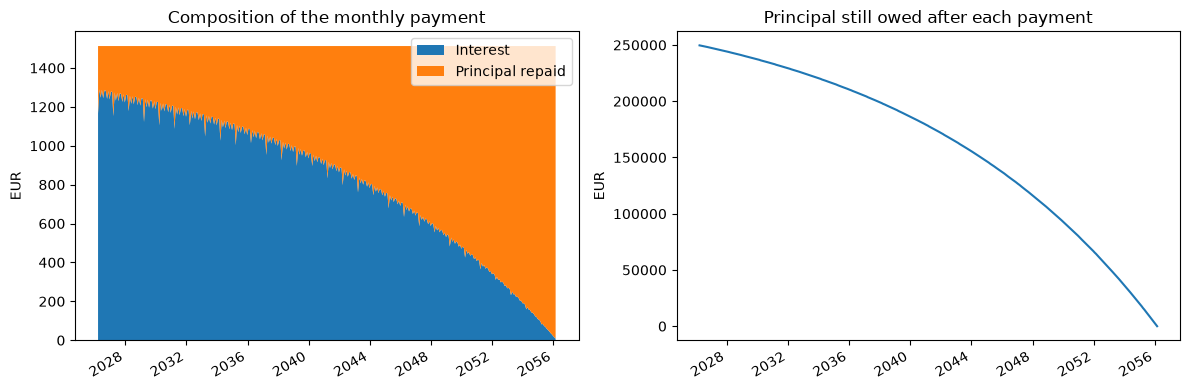
The regular payment is EUR 1,512.61. Its first interest component is EUR 1,166.67, leaving EUR 345.95 to repay principal. April’s interest rises to EUR 1,289.88 because its accrual period has 31 days. Over time the interest component falls and more of each regular payment repays principal.

This is a slow process over a 30-year mortgage. After ten years the borrower still owes EUR 209,682.45, about 84% of the original advance. After twenty years, EUR 135,741.07 remains. Total contractual interest reaches EUR 294,540.62 over the full term. Substantial balances remain exposed to interest rates and borrower default for decades, making early repayment a major driver of expected income.

The library computes an unrounded schedule; the tables display amounts to two decimal places.

Choosing when principal returns

Repayment timing changes both borrower funding and lender exposure. A bullet loan keeps the full EUR 250,000 outstanding until maturity, so each intervening payment consists of interest. A balloon loan combines regular amortization with a specified residual principal amount due at the end.

Here balloon(residual_fraction=0.25) reserves EUR 62,500 of original principal for maturity. For residual \(L\), the regular payment becomes

\[A=\frac{B_0-L a_n}{\sum_{k=1}^{n}a_k}.\]

The final receipt includes the regular payment and the residual. We keep the 6% coupon and market assumptions the same across structures to see how the timing of principal affects monthly payments, total interest, and receipt value.

repayment_choices = {
    "French": fixed,
    "Bullet": qs.Loan(
        identifier="BULLET",
        coupons=[qs.FixedRateCoupon(rate=fixed_rate)],
        repayment=qs.LoanRepaymentStructure.bullet(),
        **loan_terms,
    ),
    "25% balloon": qs.Loan(
        identifier="BALLOON",
        coupons=[qs.FixedRateCoupon(rate=fixed_rate)],
        repayment=qs.LoanRepaymentStructure.balloon(residual_fraction=0.25),
        **loan_terms,
    ),
}
repayment_comparison = []
with context:
    for label, instrument in repayment_choices.items():
        result = context.evaluate(
            trade=qs.Trade(instrument=instrument, trade_date=valuation_date),
            requests=[qs.Request.Value, qs.Request.Cashflows],
        )
        payments = result.cashflows.groupby("payment_date").amount.sum()
        interest = result.cashflows.loc[
            result.cashflows.type == "FixedRateCoupon", "amount"
        ].sum()
        repayment_comparison.append(
            {
                "Repayment": label,
                "First payment (EUR)": payments.iloc[0],
                "Final payment (EUR)": payments.iloc[-1],
                "Total interest (EUR)": interest,
                "Value of receipts (EUR)": result.price,
            }
        )
display(pd.DataFrame(repayment_comparison).set_index("Repayment"))

	First payment (EUR)	Final payment (EUR)	Total interest (EUR)	Value of receipts (EUR)
Repayment
French	1,512.61	1,512.61	294,540.62	358,742.79
Bullet	1,166.67	251,291.67	456,541.67	402,421.74
25% balloon	1,451.44	63,951.44	335,017.32	369,654.42

The bullet loan earns interest on the full principal for thirty years. Its smaller interim payments leave the borrower with the entire EUR 250,000 still to repay at maturity. The 25% balloon lowers the regular payment to EUR 1,451.44, with a final EUR 63,951.44 receipt that includes the EUR 62,500 residual.

Both structures keep principal outstanding longer than French amortization. That increases total interest and the lender’s exposure to future market rates and default. Here the 6% coupon exceeds the ESTR-discounted par rate, so retaining that balance also increases the present value of the promised receipts.

Floating interest, annual resets, and an introductory fixed period

A EURIBOR12m loan with a 1% spread earns an annual coupon equal to the applicable EURIBOR fixing plus 100 basis points. Payment frequency and reset frequency serve different purposes: this loan pays monthly, while the 12-month index resets the reference rate once a year. Each of the following twelve monthly coupons uses that observed rate.

The library takes the reset frequency and observation tenor from the index metadata. The loan’s two-business-day fixing lag places the first observation on 20 February, before our valuation date. We supply that historical fixing as 4%. Later observations come from the EURIBOR projection curve. Interest accrues over each monthly period using the loan’s Actual/360 convention.

For amortization, we choose an initial all-in rate of 5%. That input determines the agreed principal amounts. Subsequent fixings determine interest on those balances, so a reset can change the total monthly payment.

floating = qs.Loan(
    identifier="FLOATING",
    coupons=[qs.FloatingRateCoupon(index=qs.MarketIndex.EURIBOR12m, spread=0.01)],
    repayment=french,
    amortization_rate=0.05,
    **loan_terms,
)
observations = floating.coupon_fixing_requests()
for observation in observations.itertuples(index=False):
    fixing_date = qs.Date.parse(s=observation.fixing_date)
    if fixing_date < valuation_date:
        known_fixings.add(
            index=qs.MarketIndex.parse(s=observation.market_index),
            date=fixing_date,
            value=0.04,
        )
display(
    observations.rename(
        columns={
            "fixing_date": "Observation date",
            "start_date": "Index period start",
            "end_date": "Index period end",
            "market_index": "Index",
        }
    )
)

context.fixings = known_fixings
with context:
    floating_result = context.evaluate(
        trade=qs.Trade(instrument=floating, trade_date=valuation_date),
        requests=requests,
    )
floating_coupons = floating_result.cashflows.loc[
    floating_result.cashflows.type == "FloatingRateCoupon",
    ["payment_date", "fixing", "accrual_period", "amount"],
].copy()
floating_coupons["All-in coupon (%)"] = (floating_coupons.fixing + 0.01) * 100
floating_coupons["EURIBOR fixing (%)"] = floating_coupons.fixing * 100
display(
    floating_coupons.iloc[[0, 1, 11, 12, -1]][
        [
            "payment_date",
            "EURIBOR fixing (%)",
            "All-in coupon (%)",
            "accrual_period",
            "amount",
        ]
    ]
    .rename(
        columns={
            "payment_date": "Payment date",
            "amount": "Interest (EUR)",
            "accrual_period": "Accrual fraction",
        }
    )
    .style.format(
        {
            "Accrual fraction": "{:.6f}",
            "EURIBOR fixing (%)": "{:.4f}",
            "All-in coupon (%)": "{:.4f}",
            "Interest (EUR)": "{:,.2f}",
        }
    )
)

	Index	Observation date	Index period start	Index period end
0	EURIBOR12m	2026-02-20	2026-02-24	2027-02-24
1	EURIBOR12m	2027-02-22	2027-02-24	2028-02-24
2	EURIBOR12m	2028-02-22	2028-02-24	2029-02-26
3	EURIBOR12m	2029-02-22	2029-02-26	2030-02-26
4	EURIBOR12m	2030-02-21	2030-02-25	2031-02-25
5	EURIBOR12m	2031-02-20	2031-02-24	2032-02-24
6	EURIBOR12m	2032-02-20	2032-02-24	2033-02-24
7	EURIBOR12m	2033-02-22	2033-02-24	2034-02-24
8	EURIBOR12m	2034-02-22	2034-02-24	2035-02-26
9	EURIBOR12m	2035-02-22	2035-02-26	2036-02-26
10	EURIBOR12m	2036-02-21	2036-02-25	2037-02-25
11	EURIBOR12m	2037-02-20	2037-02-24	2038-02-24
12	EURIBOR12m	2038-02-22	2038-02-24	2039-02-24
13	EURIBOR12m	2039-02-22	2039-02-24	2040-02-24
14	EURIBOR12m	2040-02-22	2040-02-24	2041-02-25
15	EURIBOR12m	2041-02-21	2041-02-25	2042-02-25
16	EURIBOR12m	2042-02-20	2042-02-24	2043-02-24
17	EURIBOR12m	2043-02-20	2043-02-24	2044-02-24
18	EURIBOR12m	2044-02-22	2044-02-24	2045-02-24
19	EURIBOR12m	2045-02-22	2045-02-24	2046-02-26
20	EURIBOR12m	2046-02-22	2046-02-26	2047-02-26
21	EURIBOR12m	2047-02-21	2047-02-25	2048-02-25
22	EURIBOR12m	2048-02-20	2048-02-24	2049-02-24
23	EURIBOR12m	2049-02-22	2049-02-24	2050-02-24
24	EURIBOR12m	2050-02-22	2050-02-24	2051-02-24
25	EURIBOR12m	2051-02-22	2051-02-24	2052-02-26
26	EURIBOR12m	2052-02-22	2052-02-26	2053-02-26
27	EURIBOR12m	2053-02-20	2053-02-24	2054-02-24
28	EURIBOR12m	2054-02-20	2054-02-24	2055-02-24
29	EURIBOR12m	2055-02-22	2055-02-24	2056-02-24

	Payment date	EURIBOR fixing (%)	All-in coupon (%)	Accrual fraction	Interest (EUR)
0	2026-03-24	4.0000	5.0000	0.077778	972.22
2	2026-04-24	4.0000	5.0000	0.086111	1,074.75
22	2027-02-24	4.0000	5.0000	0.086111	1,061.93
24	2027-03-24	3.6913	4.6913	0.077778	898.89
718	2056-02-24	2.6090	3.6090	0.086111	4.19

At the second reset, the projected index is about 3.89%, giving an all-in coupon of about 4.89%. For EURIBOR’s simple-rate convention, the forward observation comes from the projection curve over the full index period:

\[F(t,T)=\frac{P_L(0,t)/P_L(0,T)-1}{\tau_L(t,T)}.\]

Here \(P_L\) contains EURIBOR projection discount factors and \(\tau_L\) is the index’s Actual/360 accrual fraction over twelve months. Deposit and swap quotes price cashflows across their quoted maturities. The discount-factor ratio extracts the return for this particular future index period.

The mortgage has thirty annual observations. Only the first fixing is already known; the remaining twenty-nine are implied by today’s projection curve. Each monthly coupon applies its annual observation plus the loan spread to that month’s accrual fraction. Future realized rates will depend on how the market evolves before each fixing date.

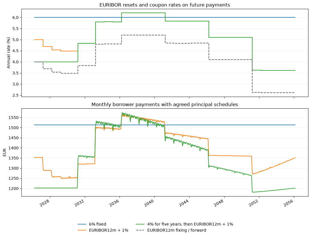
A five-year introductory fixed period changes the coupon schedule. In the next loan, the first sixty monthly periods earn 4%; the remaining periods earn EURIBOR12m plus 1%. The coupon list ends with the floating definition, which continues to maturity. The first fixed coupon supplies the initial amortization rate, giving this agreement a principal schedule based on 4%.

The upper panel shows EURIBOR fixings and the annual coupon rates resolved by the pricer. The dashed line traces the known first fixing and subsequent projected resets. After year five, the two floating coupon rates coincide. Log-linear interpolation of discount factors gives nearly constant forwards between quote pillars, and each annual observation holds until the next reset.

The lower panel shows the borrower’s monthly payments. For a French principal schedule built at initial rate \(r_0\), the payment under actual coupon \(r_i\) is

\[A_i=A_0+B_{i-1}(r_i-r_0)\tau_i.\]

Here \(A_0\) is the original level payment and \(B_{i-1}\) is that period’s agreed opening balance. The floating mortgage uses \(r_0=5\%\), so a projected all-in coupon close to 5% produces a payment close to its original instalment. The introductory-fixed mortgage uses \(r_0=4\%\); interest above that basis increases its payment after the switch. As the balance falls, the same rate difference has a smaller effect on the amount paid.

introductory_coupon = qs.FixedRateCoupon(
    rate=qs.InterestRate(
        rate=0.04,
        day_counter=qs.DayCounter.Actual360,
        compounding=qs.Compounding.Simple,
        frequency=qs.Frequency.Annual,
    )
)
floating_coupon = qs.FloatingRateCoupon(index=qs.MarketIndex.EURIBOR12m, spread=0.01)
introductory_periods = introductory_years * 12
mixed = qs.Loan(
    identifier="INTRODUCTORY-FIXED",
    coupons=[introductory_coupon] * introductory_periods + [floating_coupon],
    repayment=french,
    **loan_terms,
)
with context:
    mixed_result = context.evaluate(
        trade=qs.Trade(instrument=mixed, trade_date=valuation_date),
        requests=requests,
    )

payment_paths = pd.DataFrame(
    {
        "6% fixed": fixed_result.cashflows.groupby("payment_date").amount.sum(),
        "EURIBOR12m + 1%": floating_result.cashflows.groupby(
            "payment_date"
        ).amount.sum(),
        "4% for five years, then EURIBOR12m + 1%": mixed_result.cashflows.groupby(
            "payment_date"
        ).amount.sum(),
    }
)
display(payment_paths.iloc[[0, 11, 12, 59, 60, 119, 239, -1]])
mixed_coupons = mixed_result.cashflows.loc[
    mixed_result.cashflows["type"].isin(["FixedRateCoupon", "FloatingRateCoupon"])
].copy()
mixed_coupon_rates = pd.Series(4.0, index=payment_paths.index)
floating_periods = mixed_coupons["type"].eq("FloatingRateCoupon")
floating_dates = mixed_coupons.loc[floating_periods, "payment_date"]
mixed_coupon_rates.loc[floating_dates] = (
    mixed_coupons.loc[floating_periods, "fixing"].to_numpy() + 0.01
) * 100
coupon_paths = pd.DataFrame(
    {
        "6% fixed": pd.Series(6.0, index=fixed_payments.index),
        "EURIBOR12m + 1%": pd.Series(
            (floating_coupons.fixing.to_numpy() + 0.01) * 100,
            index=floating_coupons.payment_date,
        ),
        "4% for five years, then EURIBOR12m + 1%": mixed_coupon_rates,
    }
)
figure, axes = plt.subplots(2, 1, figsize=(11, 8.5), sharex=True)
dates = pd.to_datetime(payment_paths.index)
for label in payment_paths:
    axes[0].step(dates, coupon_paths[label], where="post", label=label)
    axes[1].plot(dates, payment_paths[label], label=label)
axes[0].step(
    dates,
    floating_coupons.fixing.to_numpy() * 100,
    where="post",
    color="0.35",
    linestyle="--",
    label="EURIBOR12m fixing / forward",
)
axes[0].set(
    title="EURIBOR resets and coupon rates on future payments", ylabel="Annual rate (%)"
)
axes[1].set(
    title="Monthly borrower payments with agreed principal schedules", ylabel="EUR"
)
for axis in axes:
    axis.grid(axis="y", alpha=0.2)
figure.legend(
    handles=axes[0].get_lines(),
    loc="lower center",
    bbox_to_anchor=(0.5, 0.02),
    ncol=2,
    frameon=False,
)
figure.autofmt_xdate()
figure.tight_layout(rect=(0, 0.12, 1, 1))
plt.show()

	6% fixed	EURIBOR12m + 1%	4% for five years, then EURIBOR12m + 1%
payment_date
2026-03-24	1,512.61	1,352.95	1,201.77
2027-02-24	1,512.61	1,352.95	1,201.77
2027-03-24	1,512.61	1,293.81	1,201.77
2031-02-24	1,512.61	1,251.82	1,201.77
2031-03-24	1,512.61	1,322.26	1,347.57
2036-02-25	1,512.61	1,493.77	1,508.55
2046-02-26	1,512.61	1,445.38	1,390.50
2056-02-24	1,512.61	1,351.34	1,201.37

Floating coupons can also have an all-in floor and cap. For a 2% floor and 4.5% cap, the coupon is \(\min(4.5\%,\max(2\%,L+1\%))\), where \(L\) is the index observation. The initial 4% fixing would otherwise produce a 5% coupon, so the cap limits the first year’s interest income.

OptionEmbeddedCoupon accepts the same PayoffOps expression tree as Rust. Index is the resolved fixing; arithmetic, min, and max combine expressions. We include the lending margin inside the expression so the bounds apply to the all-in rate. The coupon’s separate spread parameter would be added after the payoff. The same operations can express gearing, for example (2 * qs.PayoffOps.Index + 0.005).max(0.02).

LoanPricer applies these bounds to the resolved index observations. The result shows the projected cash payments under those rates. A valuation of the embedded interest-rate option’s time value would additionally require a volatility model.

bounded = qs.Loan(
    identifier="FLOOR-AND-CAP",
    coupons=[
        qs.OptionEmbeddedCoupon(
            index=qs.MarketIndex.EURIBOR12m,
            payoff=(qs.PayoffOps.Index + 0.01).max(0.02).min(0.045),
            day_counter=qs.DayCounter.Actual360,
        )
    ],
    repayment=french,
    amortization_rate=0.05,
    **loan_terms,
)
with context:
    bounded_result = context.evaluate(
        trade=qs.Trade(instrument=bounded, trade_date=valuation_date),
        requests=[qs.Request.Value, qs.Request.Cashflows],
    )
display(
    pd.DataFrame(
        {
            "Unbounded floating": floating_result.cashflows.groupby(
                "payment_date"
            ).amount.sum(),
            "2% floor, 4.5% cap": bounded_result.cashflows.groupby(
                "payment_date"
            ).amount.sum(),
        }
    ).iloc[[0, 11, 12, -1]]
)

	Unbounded floating	2% floor, 4.5% cap
payment_date
2026-03-24	1,352.95	1,255.73
2027-02-24	1,352.95	1,246.76
2027-03-24	1,293.81	1,257.15
2056-02-24	1,351.34	1,351.34

Present value and the coupon that lends at par

A loan’s value depends on the timing of its income. For discount factors \(D(0,t_i)\) and future receipts \(C_i\), the lender’s receipt value is

\[V_{\mathrm{receipts}}=\sum_i D(0,t_i)\,\mathbb{E}[C_i].\]

The price returned by the loan pricer is this value of future receipts. At origination the lender also advances EUR 250,000, giving an initial net value of \(V_{\mathrm{receipts}}-250{,}000\). Payment dates strictly after the valuation date enter the receipt value. Our example starts on the valuation date, so the full advance occurs today.

With a 6% fixed coupon and the selected ESTR discount curve, the loan trades at a premium to its original principal. The nominal interest total and present value answer different financial questions: the former measures currency received over the life of the loan, while the latter accounts for when it arrives.

origination_values = []
for label, result in [
    ("6% fixed", fixed_result),
    ("EURIBOR12m + 1%", floating_result),
    ("Introductory fixed", mixed_result),
]:
    origination_values.append(
        {
            "Agreement": label,
            "Value of receipts (EUR)": result.price,
            "Advance today (EUR)": principal,
            "Lender value after advance (EUR)": result.price - principal,
        }
    )
display(pd.DataFrame(origination_values).set_index("Agreement"))

	Value of receipts (EUR)	Advance today (EUR)	Lender value after advance (EUR)
Agreement
6% fixed	358,742.79	250,000.00	108,742.79
EURIBOR12m + 1%	331,004.10	250,000.00	81,004.10
Introductory fixed	320,936.48	250,000.00	70,936.48

Selecting a different discount policy

Assign a qs.FixedIncomeDiscountPolicy to context.fixed_income_policy, then call context.evaluate(...) as usual. The mapping selects a discount curve by payment currency. Its index must identify a curve configured in context.curves; assigning the policy does not create that curve. Our market already contains both ESTR and EURIBOR12m, so we can compare them directly.

The following cell selects EURIBOR12m for EUR receipts and restores ESTR for the remaining study. The fixed loan’s payments stay the same; only their present value changes. For a floating loan, the coupon’s index still selects its projection curve. context.csa_policy continues to specify the collateral convention used for market construction.

You can also pass fixed_income_policy=... when creating PricingContext. Setting context.fixed_income_policy = None restores the default policy based on the context’s base currency and curve. The funding section below applies the same mapping to a composite cost-of-funds curve.

euribor_discount_policy = qs.FixedIncomeDiscountPolicy(
    discount_curve_by_currency={qs.Currency.EUR: qs.MarketIndex.EURIBOR12m}
)
context.fixed_income_policy = euribor_discount_policy
try:
    with context:
        fixed_on_euribor = context.evaluate(
            qs.Trade(fixed, valuation_date, qs.Side.LongReceive),
            [qs.Request.Value, qs.Request.Cashflows],
        )
finally:
    context.fixed_income_policy = estr_policy

display(
    pd.DataFrame(
        {"Value of receipts (EUR)": [fixed_result.price, fixed_on_euribor.price]},
        index=pd.Index(["ESTR", "EURIBOR12m"], name="Discount curve"),
    )
)

	Value of receipts (EUR)
Discount curve
ESTR	358,742.79
EURIBOR12m	307,937.61

FairRate solves the coupon or floating spread that makes the value of receipts equal to the value of the advance. There are two useful ways to pose that problem. An existing principal schedule can be retained while changing its coupon. A new loan can instead have its amortization recalculated for each candidate rate.

rebuild_amortization_for_fair_rate selects between those two assumptions. With False, the solver keeps the agreed principal amounts. With True, it rebuilds the French payment using the trial fixed coupon, or the first observed index rate plus the trial floating spread. The settings can give different par rates because they change the timing of principal repayments. The library supports this solve at or before origination for uniform fixed or unbounded floating coupons.

We set the amortization option with PricerConfiguration.loan(...) in the context before calling context.evaluate(...). The context dispatches directly to the Rust loan pricer and supplies its fixed-income discount policy. The finally block restores the default loan configuration for the remaining study.

fair_rate_comparison = []
try:
    with context:
        for rebuild, schedule in [
            (False, "Keep the agreed principal schedule"),
            (True, "Rebuild principal at the trial rate"),
        ]:
            context.pricer_configurations = [qs.PricerConfiguration.loan(
                rebuild_amortization_for_fair_rate=rebuild,
            )]
            fixed_fair = context.evaluate(
                trade=qs.Trade(instrument=fixed, trade_date=valuation_date),
                requests=[qs.Request.FairRate(0)],
            ).fair_rate
            floating_fair = context.evaluate(
                trade=qs.Trade(instrument=floating, trade_date=valuation_date),
                requests=[qs.Request.FairRate(0)],
            ).fair_rate
            fair_rate_comparison.append(
                {
                    "Principal assumption": schedule,
                    "Par fixed coupon (%)": fixed_fair * 100,
                    "Par EURIBOR spread (bp)": floating_fair * 10_000,
                }
            )
finally:
    context.pricer_configurations = [loan_configuration]
display(
    pd.DataFrame(fair_rate_comparison)
    .set_index("Principal assumption")
    .style.format("{:,.6f}")
)

	Par fixed coupon (%)	Par EURIBOR spread (bp)
Principal assumption
Keep the agreed principal schedule	2.958781	-133.298963
Rebuild principal at the trial rate	2.958477	-131.947212

In this illustrative market, the EURIBOR projection curve produces a higher benchmark coupon than the ESTR-discounted par lending rate requires. The par floating spread is consequently negative. It is the adjustment to the benchmark needed under these particular cashflow and discount assumptions. The fixed solution is an annual coupon; the floating solution is a margin added to EURIBOR.

Valuing the loan against the lender’s cost of funds

A lender funding an asset at EURIBOR plus a treasury spread needs the loan’s income to cover both components. We can express that funding hurdle as a discount curve and ask what the agreed receipts are worth on that basis. This also gives us the coupon or lending margin required to cover funding at origination.

We use the existing EURIBOR12m curve as the benchmark and introduce a separate funding spread term structure. Its continuously compounded zero spreads rise from 50 bp today to 100 bp at five years, 125 bp at twenty years, and 140 bp at thirty years. A final pillar at thirty-five years is 150 bp. Interpolation is linear on Actual/360 time. These are illustrative treasury assumptions; the spread is charged over the EURIBOR benchmark.

For spread \(s(T)\) and year fraction \(\tau(0,T)\), the composite curve has

\[D_{\mathrm{funding}}(0,T) =D_{\mathrm{EURIBOR}}(0,T)\,D_{\mathrm{spread}}(0,T) =D_{\mathrm{EURIBOR}}(0,T)\,e^{-s(T)\tau(0,T)}.\]

Equivalently, the continuously compounded zero rate is \(z_{\mathrm{funding}}(T)=z_{\mathrm{EURIBOR}}(T)+s(T)\). The EURIBOR zero rate here is obtained from its discount factor on the same time basis. This preserves the compounding conventions of the underlying deposit and swap quotes.

The spread and composite curves are CurveConfiguration entries in the same curves list as ESTR and EURIBOR. Pricing requests build their dependencies, including under each scenario. Assigning a FixedIncomeDiscountPolicy to context.fixed_income_policy selects the funding curve for the next context.evaluate(...) call. The same loan agreements and pricing requests produce the funding values below.

cost_of_funds_index = qs.MarketIndex.other(name="COSTOFFUNDS")
funding_tenors = [
    qs.Period(length=0, units=qs.TimeUnit.Days),
    *[
        qs.Period(length=years, units=qs.TimeUnit.Years)
        for years in [1, 5, 10, 20, 30, 35]
    ],
]
funding_spreads = [0.0050, 0.0075, 0.0100, 0.0115, 0.0125, 0.0140, 0.0150]
display(
    pd.DataFrame(
        {
            "Tenor": [str(tenor) for tenor in funding_tenors],
            "Continuous zero funding spread (bp)": [
                rate * 10_000 for rate in funding_spreads
            ],
        }
    ).set_index("Tenor")
)

funding_spread_index = qs.MarketIndex.other(name="FUNDINGSPREAD")
spread_configuration = qs.CurveConfiguration(
    market_index=funding_spread_index,
    day_counter=qs.DayCounter.Actual360,
    interpolator=qs.Interpolator.Linear,
    enable_extrapolation=False,
    quotes=[f"ZeroRate_EUR_FUNDINGSPREAD_{tenor}" for tenor in funding_tenors],
)
funding_configuration = qs.CurveConfiguration.composite(market_index=cost_of_funds_index, base_index=qs.MarketIndex.EURIBOR12m, spread_index=funding_spread_index)
funding_policy = qs.FixedIncomeDiscountPolicy(
    discount_curve_by_currency={qs.Currency.EUR: cost_of_funds_index}
)
benchmark_policy = qs.FixedIncomeDiscountPolicy(
    discount_curve_by_currency={qs.Currency.EUR: qs.MarketIndex.EURIBOR12m}
)
funding_quote_records = [
    {"identifier": identifier, **dict(zip(("mid", "bid", "ask"), market.quotes.levels(identifier)))}
    for identifier in market.quotes.identifiers()
]
funding_quote_records += [
    {"identifier": f"ZeroRate_EUR_FUNDINGSPREAD_{tenor}", "mid": rate}
    for tenor, rate in zip(funding_tenors, funding_spreads)
]
context.quotes = qs.QuoteStore.from_dict({"reference_date": str(valuation_date), "quotes": funding_quote_records})
context.curves = market.curves + [spread_configuration, funding_configuration]
context.fixed_income_policy = funding_policy

funding_values = []
funding_base_results = {}
with context:
    for label, instrument in [("6% fixed", fixed), ("EURIBOR12m + 1%", floating)]:
        for discount_basis, policy in [
            ("ESTR", estr_policy),
            ("EURIBOR12m", benchmark_policy),
            ("EURIBOR12m + funding spread", funding_policy),
        ]:
            context.fixed_income_policy = policy
            result = context.evaluate(
                trade=qs.Trade(instrument=instrument, trade_date=valuation_date),
                requests=[
                    qs.Request.Value,
                    qs.Request.FairRate(0),
                    qs.Request.Sensitivities,
                ],
            )
            if discount_basis == "EURIBOR12m + funding spread":
                funding_base_results[label] = result
            funding_values.append(
                {
                    "Loan": label,
                    "Discount basis": discount_basis,
                    "Value of receipts (EUR)": result.price,
                    "Value after advance (EUR)": result.price - principal,
                    "Par fixed coupon (%)": (
                        result.fair_rate * 100 if instrument is fixed else None
                    ),
                    "Par EURIBOR margin (bp)": (
                        result.fair_rate * 10_000 if instrument is floating else None
                    ),
                }
            )
display(
    pd.DataFrame(funding_values)
    .set_index(["Loan", "Discount basis"])
    .style.format("{:,.2f}", na_rep="—")
)

	Continuous zero funding spread (bp)
Tenor
0D	50.00
1Y	75.00
5Y	100.00
10Y	115.00
20Y	125.00
30Y	140.00
35Y	150.00

		Value of receipts (EUR)	Value after advance (EUR)	Par fixed coupon (%)	Par EURIBOR margin (bp)
Loan	Discount basis
6% fixed	ESTR	358,742.79	108,742.79	2.96	—
	EURIBOR12m	307,937.61	57,937.61	4.19	—
	EURIBOR12m + funding spread	267,842.00	17,842.00	5.38	—
EURIBOR12m + 1%	ESTR	331,004.10	81,004.10	—	-133.30
	EURIBOR12m	283,729.77	33,729.77	—	-8.39
	EURIBOR12m + funding spread	246,392.19	-3,607.81	—	112.83

The fixed mortgage’s receipt value falls from EUR 358,742.79 under ESTR discounting to EUR 303,807.00 on EURIBOR and EUR 264,555.88 after the funding spread. Its funding-based par coupon is about 5.49%. At the agreed 6% coupon, the receipt value exceeds the original advance by EUR 14,555.88.

For the floating mortgage, the funding-based par margin is 112.22 bp. Its agreed 100 bp margin falls short of that hurdle: receipts are worth EUR 246,596.61, leaving a value of EUR -3,403.39 after the advance. A spread that covers funding at the front of the curve can be insufficient over a thirty-year income stream when treasury funding spreads rise with maturity.

The fair-rate calculations retain each agreed principal schedule, using the default rebuild_amortization_for_fair_rate=False. Prepayment and borrower recovery will change expected receipts in the following sections.

Funding-spread sensitivities

A wider treasury funding spread reduces the value of each remaining receipt. The effect depends on when principal and interest return: a spread pillar near the mortgage’s large later balances carries more exposure than one near its last small payments. Linear interpolation distributes that exposure between the neighbouring funding pillars.

We request qs.Request.Sensitivities with the funding discount policy selected. The result includes derivatives with respect to the original funding zero spreads, labelled ZeroRate_EUR_FUNDINGSPREAD_<tenor>. A value is EUR per unit decimal spread; multiplying by 0.0001 gives the approximate EUR value change for a +1 bp increase in that pillar, holding other inputs fixed.

The first table separates funding spreads from the benchmark quotes. The next table and chart isolate each funding-spread maturity. Adding those bucket sensitivities gives the first-order effect of a parallel +1 bp funding move.

def curve_input_family(pillar):
    if "FUNDINGSPREAD" in pillar:
        return "Funding zero spreads"
    if "EURIBOR" in pillar:
        return "EURIBOR market quotes"
    return "ESTR market quotes"


context.fixed_income_policy = funding_policy
funding_risks = []
with context:
    for label, instrument in [("6% fixed", fixed), ("EURIBOR12m + 1%", floating)]:
        result = context.evaluate(
            trade=qs.Trade(instrument=instrument, trade_date=valuation_date),
            requests=[qs.Request.Sensitivities],
        )
        risk = result.sensitivities.copy()
        risk["Loan"] = label
        risk["EUR change for +1bp"] = risk.value * 0.0001
        risk["Curve input"] = risk["pillar"].map(curve_input_family)
        funding_risks.append(risk)
funding_risk = pd.concat(funding_risks, ignore_index=True)
funding_pv01 = funding_risk.pivot_table(
    index="Curve input",
    columns="Loan",
    values="EUR change for +1bp",
    aggfunc="sum",
    fill_value=0,
)
display(funding_pv01.style.format("{:+,.2f}"))

funding_pillar_labels = [
    f"ZeroRate_EUR_FUNDINGSPREAD_{tenor}" for tenor in funding_tenors
]
funding_spread_sensitivities = (
    funding_risk.loc[funding_risk.pillar.isin(funding_pillar_labels)]
    .pivot(index="pillar", columns="Loan", values="EUR change for +1bp")
    .reindex(funding_pillar_labels)
)
funding_spread_sensitivities.index = pd.Index(
    [str(tenor) for tenor in funding_tenors], name="Funding spread tenor"
)
display(funding_spread_sensitivities.style.format("{:+,.4f}"))

axis = funding_spread_sensitivities.plot.bar(
    figsize=(10, 4.5), color=["#2864a5", "#e69834"]
)
axis.axhline(0, color="black", linewidth=0.8)
axis.set(
    ylabel="Approximate EUR value change for +1 bp",
    xlabel="Funding zero-spread pillar",
    title="Mortgage exposure to each funding-spread maturity",
)
axis.legend(title="Loan")
plt.xticks(rotation=0)
plt.tight_layout()
plt.show()

Loan	6% fixed	EURIBOR12m + 1%
Curve input
ESTR market quotes	-4.20	+0.34
EURIBOR market quotes	-279.24	-8.14
Funding zero spreads	-295.46	-275.84

Loan	6% fixed	EURIBOR12m + 1%
Funding spread tenor
0D	-0.2960	-0.2647
1Y	-8.1762	-6.8757
5Y	-33.3653	-29.6330
10Y	-83.3903	-83.1543
20Y	-115.4609	-107.9241
30Y	-54.7719	-47.9881
35Y	+0.0000	+0.0000

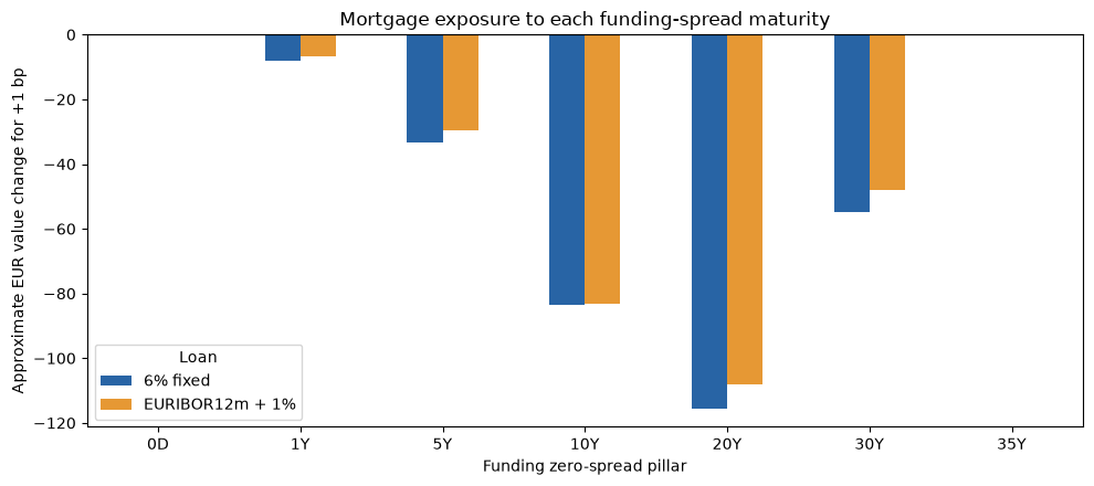
The fixed mortgage loses about EUR 285 for a +1 bp move across EURIBOR quotes and EUR 290 for +1 bp across the funding zero spreads. For the floating mortgage, the corresponding EURIBOR exposure is about EUR -7: higher projected interest offsets much of the discounting effect. The same funding spread move still reduces its value by about EUR 274.

A smaller ESTR exposure remains because EURIBOR swaps are calibrated using ESTR discount factors. Changing an ESTR quote can therefore change the calibrated EURIBOR curve and the composite funding value. The sensitivity request follows that calibration dependency as well as the direct cashflow effects.

Scenarios: benchmark rates and funding pressure

Two changes matter to the funded lender. A move in EURIBOR changes the benchmark component of discounting and the floating coupons whose fixings are still in the future. A wider treasury spread increases the funding hurdle for every remaining receipt. We can examine each channel, then combine them in a funding stress.

A qs.Shock with target="EURIBOR12m" selects the EURIBOR quote pillars. An absolute value=0.01 adds 100 bp to each quote, and the view bootstraps a fresh benchmark curve. These are parallel quote shocks; the calibrated zero and forward rates move according to the curve construction. The funding spread curve uses direct zero-rate quotes, so a funding shock adds directly to each of its spread pillars before composition.

qs.Scenario(shocks=[...]) combines the two shocks. In with context, scenario:, pricing uses a temporary view of the context’s market inputs. The view constructs the requested curves and their dependencies, and keeps its own AD state for sensitivities. The context retains its base inputs and curves. Exiting the scope, including through an exception, releases the view. The same context can then be used for another scenario or a base valuation. The funding-spread selector targets the same labelled zero pillars used by the sensitivity request.

We keep the loan contracts and known fixings. In particular, the floating loan’s first annual EURIBOR fixing remains 4%, and its existing principal amounts stay in place. Profit or loss is the change in the funding-discounted receipt value relative to the base market.

market_scenarios = [
    ("Base market", 0, 0),
    ("EURIBOR falls 100 bp", -100, 0),
    ("EURIBOR rises 100 bp", 100, 0),
    ("Funding spread widens 50 bp", 0, 50),
    ("EURIBOR +100 bp; funding +50 bp", 100, 50),
]
scenario_values = []
for scenario_name, benchmark_shift_bp, funding_shift_bp in market_scenarios:
    scenario = qs.Scenario(
        shocks=[
            qs.Shock(
                target="EURIBOR12m",
                value=benchmark_shift_bp / 10_000,
                shock_type=qs.ScenarioType.Absolute,
            ),
            qs.Shock(
                target="FUNDINGSPREAD",
                value=funding_shift_bp / 10_000,
                shock_type=qs.ScenarioType.Absolute,
            ),
        ]
    )
    with context, scenario:
        for label, instrument in [("6% fixed", fixed), ("EURIBOR12m + 1%", floating)]:
            result = context.evaluate(
                trade=qs.Trade(instrument=instrument, trade_date=valuation_date),
                requests=[qs.Request.Value, qs.Request.Cashflows],
            )
            coupons = result.cashflows.loc[
                result.cashflows.type.isin(["FixedRateCoupon", "FloatingRateCoupon"])
            ]
            scenario_values.append(
                {
                    "Scenario": scenario_name,
                    "Loan": label,
                    "EURIBOR quote shift (bp)": benchmark_shift_bp,
                    "Funding spread shift (bp)": funding_shift_bp,
                    "Projected interest (EUR)": coupons.amount.sum(),
                    "Funding value (EUR)": result.price,
                    "Profit or loss (EUR)": result.price
                    - funding_base_results[label].price,
                    "First-order funding effect (EUR)": (
                        funding_pv01.loc["Funding zero spreads", label]
                        * funding_shift_bp
                        if benchmark_shift_bp == 0
                        else None
                    ),
                }
            )
scenario_table = pd.DataFrame(scenario_values)
display(
    scenario_table.set_index(["Scenario", "Loan"]).style.format("{:,.2f}", na_rep="—")
)

scenario_pnl = scenario_table.pivot(
    index="Scenario", columns="Loan", values="Profit or loss (EUR)"
).reindex([name for name, _, _ in market_scenarios][1:])
ax = scenario_pnl.plot.barh(figsize=(10, 4.5), color=["#2864a5", "#e69834"])
ax.axvline(0, color="black", linewidth=0.8)
ax.set_xlabel("Change in funding-discounted value (EUR)")
ax.set_ylabel("")
ax.set_title("The same agreements under changed funding conditions")
ax.legend(title="Loan", loc="upper center", bbox_to_anchor=(0.5, -0.18), ncol=2)
plt.tight_layout()
plt.show()
context.curves = market.curves
context.fixed_income_policy = estr_policy

		EURIBOR quote shift (bp)	Funding spread shift (bp)	Projected interest (EUR)	Funding value (EUR)	Profit or loss (EUR)	First-order funding effect (EUR)
Scenario	Loan
Base market	6% fixed	0.00	0.00	294,540.62	267,842.00	0.00	-0.00
	EURIBOR12m + 1%	0.00	0.00	252,764.52	246,392.19	0.00	-0.00
EURIBOR falls 100 bp	6% fixed	-100.00	0.00	294,540.62	298,322.12	30,480.12	—
	EURIBOR12m + 1%	-100.00	0.00	208,548.05	247,196.34	804.16	—
EURIBOR rises 100 bp	6% fixed	100.00	0.00	294,540.62	242,137.54	-25,704.45	—
	EURIBOR12m + 1%	100.00	0.00	296,981.41	245,567.96	-824.22	—
Funding spread widens 50 bp	6% fixed	0.00	50.00	294,540.62	253,677.18	-14,164.82	-14,773.02
	EURIBOR12m + 1%	0.00	50.00	252,764.52	233,162.50	-13,229.69	-13,792.00
EURIBOR +100 bp; funding +50 bp	6% fixed	100.00	50.00	294,540.62	230,019.18	-37,822.82	—
	EURIBOR12m + 1%	100.00	50.00	296,981.41	233,236.72	-13,155.47	—

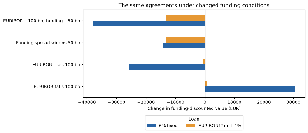
The fixed mortgage keeps its EUR 294,540.62 of contractual interest in every scenario. A 100 bp EURIBOR increase lowers its funding-discounted value by EUR 26,281.87. The floating mortgage loses only EUR 755.23 under that same move: its future annual resets raise coupon income and offset much of the increased benchmark funding cost. The first year’s known fixing remains unchanged.

Funding-spread widening has no matching increase in borrower coupons. A 50 bp widening leaves projected interest unchanged and reduces the fixed and floating receipt values by EUR 13,889.63 and EUR 13,122.83 respectively. When EURIBOR also rises 100 bp, floating interest over the term increases to EUR 305,048.19, while its funding-discounted receipt value is EUR 233,640.77.

These scenarios retain the agreed principal schedules. The refinancing example below adds the borrower’s early-repayment response to the benchmark move.

Early repayment and the life of the income stream

A borrower who prepays returns principal earlier and reduces the interest the lender will receive later. Conditional prepayment rate, or CPR, expresses the annual rate of early principal repayment on the balance that remains after scheduled amortization.

For a regular monthly interval, the library converts annual CPR \(c\) to a monthly conditional probability

\[\pi=1-(1-c)^{1/12}.\]

With 25% annual CPR, this is about 2.37% per month. The pricer first pays scheduled principal \(Q_i\), then applies \(\pi_i\) to the remaining balance. Future scheduled interest and principal are weighted by the fraction expected to remain. This produces an expected balance path while retaining the agreed contractual terms.

The prepayment interval has its own clock: a full monthly interval uses \(1/12\) year, and partial or irregular intervals use Actual/365. Coupon interest in our agreement continues to use Actual/360.

prepayment_models = {
    "Scheduled payments only": qs.PrepaymentModelConfiguration.no_prepayment(),
    "12% annual CPR": qs.PrepaymentModelConfiguration.constant_annual_cpr(cpr=0.12),
    "25% annual CPR": qs.PrepaymentModelConfiguration.constant_annual_cpr(cpr=0.25),
}
prepayment_results = {}
prepayment_comparison = []
with context:
    for label, model in prepayment_models.items():
        instrument = qs.Loan(
            identifier=label,
            coupons=[qs.FixedRateCoupon(rate=fixed_rate)],
            repayment=french,
            prepayment=model,
            **loan_terms,
        )
        result = context.evaluate(
            trade=qs.Trade(instrument=instrument, trade_date=valuation_date),
            requests=requests,
        )
        prepayment_results[label] = result
        principal_receipts = result.cashflows.loc[result.cashflows.type == "Redemption"]
        average_life = (
            sum(
                row.amount
                * qs.DayCounter.Actual365.year_fraction(
                    start=valuation_date, end=qs.Date.parse(s=row.payment_date)
                )
                for row in principal_receipts.itertuples(index=False)
            )
            / principal
        )
        prepayment_comparison.append(
            {
                "Prepayment assumption": label,
                "Expected principal life (years)": average_life,
                "Expected interest (EUR)": result.cashflows.loc[
                    result.cashflows.type == "FixedRateCoupon", "amount"
                ].sum(),
                "Value of receipts (EUR)": result.price,
            }
        )
display(pd.DataFrame(prepayment_comparison).set_index("Prepayment assumption"))

figure, axis = plt.subplots(figsize=(10, 4))
for label, result in prepayment_results.items():
    principal_receipts = (
        result.cashflows.loc[result.cashflows.type == "Redemption"]
        .groupby("payment_date")
        .amount.sum()
    )
    balance = principal - principal_receipts.cumsum()
    axis.plot(pd.to_datetime(balance.index), balance, label=label)
axis.set(
    title="Expected outstanding principal under different CPR assumptions", ylabel="EUR"
)
axis.legend()
figure.autofmt_xdate()
figure.tight_layout()
plt.show()

	Expected principal life (years)	Expected interest (EUR)	Value of receipts (EUR)
Prepayment assumption
Scheduled payments only	19.37	294,540.62	358,742.79
12% annual CPR	6.68	101,591.86	293,586.91
25% annual CPR	3.34	50,735.26	273,546.04

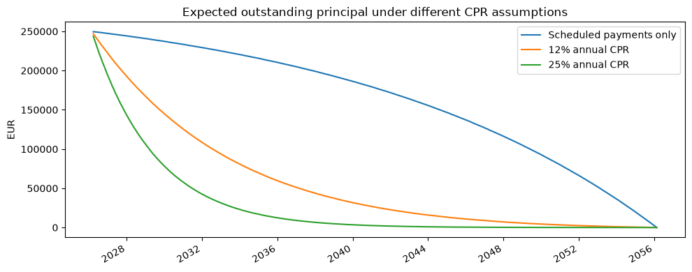
The expected principal life is the average time at which each euro of principal returns, weighted by its repayment amount. Scheduled amortization gives this mortgage a principal life of 19.37 years. At 12% annual CPR it falls to 6.68 years; at 25% CPR it falls to 3.34 years, despite the same thirty-year contractual term.

At 25% CPR, expected interest falls from EUR 294,540.62 to EUR 50,735.26, and the receipt value falls from EUR 358,742.79 to EUR 273,546.04. The lender receives principal much sooner but loses decades of above-market fixed coupon income.

The library also supports a dated CPR curve through PrepaymentModelConfiguration.dated_annual_cpr. It uses the latest annual CPR whose effective date has been reached at the start of the interval, zero before the first date, and the last supplied rate for subsequent intervals. This can represent a seasoning pattern or an expected change in borrower behaviour.

Prepayment changes the par lending rate and market sensitivity

We now compare the fixed, floating, and introductory-fixed agreements against the same EURIBOR-plus-funding-spread curve used above. For each agreement we retain its original principal schedule and change only the prepayment assumption. Keeping the shaped funding curve makes the effect of earlier repayment on the par lending hurdle visible; under a nearly flat ESTR curve, constant CPR can have very little effect on the par fixed coupon even while materially reducing value and duration.

FairRate includes the prepayment model in every trial valuation. With the default rebuild_amortization_for_fair_rate=False, it changes the uniform fixed coupon or floating spread without rebuilding the contractual principal amounts. The table reports the resulting par rate and its change in basis points from no prepayment. These are alternative lending terms, not changes to the borrower’s agreed coupon.

Targeted fair rates: qs.Request.FairRate(0) selects the first contiguous coupon segment; qs.Request.FairRate(1) selects the second. For the introductory loan the latter bootstraps the first coupon, repays remaining capital at that prefix end, locks the coupon, then solves the later spread. Each evaluation returns one scalar fair_rate. The comparison below keeps its original value and risk columns; the following cell demonstrates both segment requests.

The second table shows signed EUR PV01: the first-order value change for a parallel +1 bp move in each named group of market inputs. The change columns subtract the corresponding no-prepayment exposure. These are sensitivities of the original agreed loan, not derivatives of the solved fair rate and not sensitivities to CPR. For constant CPR, repayment probabilities do not respond to market quotes; the refinancing example below adds that response. The first EURIBOR fixing remains known and unchanged.

prepayment_agreements = {
    "6% fixed": fixed,
    "EURIBOR12m + 1%": floating,
    "Introductory fixed": mixed,
}
prepayment_funding_loans = {}
for loan_label, agreement in prepayment_agreements.items():
    for prepayment_label, model in prepayment_models.items():
        terms = agreement.to_dict()
        terms["identifier"] = f"{loan_label}: {prepayment_label}"
        terms["prepayment"] = model.to_dict()
        prepayment_funding_loans[(loan_label, prepayment_label)] = qs.Loan.from_dict(
            obj=terms
        )

prepayment_funding_results = {}
prepayment_rate_rows = []
prepayment_risk_rows = []
context.curves = market.curves + [spread_configuration, funding_configuration]
context.fixed_income_policy = funding_policy
try:
    with context:
        for (
            loan_label,
            prepayment_label,
        ), instrument in prepayment_funding_loans.items():
            pricing_requests = [qs.Request.Value, qs.Request.Sensitivities]
            if loan_label != "Introductory fixed":
                pricing_requests.append(qs.Request.FairRate(0))
            result = context.evaluate(
                trade=qs.Trade(instrument=instrument, trade_date=valuation_date),
                requests=pricing_requests,
            )
            prepayment_funding_results[(loan_label, prepayment_label)] = result
            prepayment_rate_rows.append(
                {
                    "Loan": loan_label,
                    "Prepayment assumption": prepayment_label,
                    "Funding value (EUR)": result.price,
                    "Par fixed coupon (%)": (
                        result.fair_rate * 100 if loan_label == "6% fixed" else None
                    ),
                    "Par EURIBOR margin (bp)": (
                        result.fair_rate * 10_000
                        if loan_label == "EURIBOR12m + 1%"
                        else None
                    ),
                    "Fair-rate support": (
                        "Separate indexed requests"
                        if loan_label == "Introductory fixed"
                        else "Native FairRate"
                    ),
                }
            )
            risk = result.sensitivities
            prepayment_risk_rows.append(
                {
                    "Loan": loan_label,
                    "Prepayment assumption": prepayment_label,
                    "ESTR PV01 (EUR)": risk.loc[
                        risk.pillar.str.contains("ESTR"), "value"
                    ].sum()
                    * 0.0001,
                    "EURIBOR PV01 (EUR)": risk.loc[
                        risk.pillar.str.contains("EURIBOR"), "value"
                    ].sum()
                    * 0.0001,
                    "Funding spread PV01 (EUR)": risk.loc[
                        risk.pillar.str.contains("FUNDINGSPREAD"), "value"
                    ].sum()
                    * 0.0001,
                }
            )
finally:
    context.curves = market.curves
    context.fixed_income_policy = estr_policy

prepayment_rate_table = pd.DataFrame(prepayment_rate_rows).set_index(
    ["Loan", "Prepayment assumption"]
)
prepayment_rate_baseline = prepayment_rate_table.xs("Scheduled payments only", level=1)
prepayment_rate_table["Change in par fixed coupon (bp)"] = (
    prepayment_rate_table["Par fixed coupon (%)"]
    - prepayment_rate_table.index.get_level_values("Loan").map(
        prepayment_rate_baseline["Par fixed coupon (%)"]
    )
) * 100
prepayment_rate_table["Change in par EURIBOR margin (bp)"] = prepayment_rate_table[
    "Par EURIBOR margin (bp)"
] - prepayment_rate_table.index.get_level_values("Loan").map(
    prepayment_rate_baseline["Par EURIBOR margin (bp)"]
)
display(
    prepayment_rate_table.style.format(
        {
            "Funding value (EUR)": "{:,.2f}",
            "Par fixed coupon (%)": "{:.6f}",
            "Par EURIBOR margin (bp)": "{:.4f}",
            "Change in par fixed coupon (bp)": "{:+.4f}",
            "Change in par EURIBOR margin (bp)": "{:+.4f}",
        },
        na_rep="Not applicable",
    )
)

prepayment_risk_table = pd.DataFrame(prepayment_risk_rows).set_index(
    ["Loan", "Prepayment assumption"]
)
for column in list(prepayment_risk_table.columns):
    baseline = prepayment_risk_table[column].xs("Scheduled payments only", level=1)
    prepayment_risk_table[f"Change in {column}"] = prepayment_risk_table[
        column
    ] - prepayment_risk_table.index.get_level_values("Loan").map(baseline)
display(prepayment_risk_table.style.format("{:+,.2f}"))

		Funding value (EUR)	Par fixed coupon (%)	Par EURIBOR margin (bp)	Fair-rate support	Change in par fixed coupon (bp)	Change in par EURIBOR margin (bp)
Loan	Prepayment assumption
6% fixed	Scheduled payments only	267,842.00	5.380956	Not applicable	Native FairRate	+0.0000	Not applicable
	12% annual CPR	262,938.12	4.997355	Not applicable	Native FairRate	-38.3601	Not applicable
	25% annual CPR	259,197.51	4.740332	Not applicable	Native FairRate	-64.0624	Not applicable
EURIBOR12m + 1%	Scheduled payments only	246,392.19	Not applicable	112.8342	Native FairRate	Not applicable	+0.0000
	12% annual CPR	249,951.45	Not applicable	100.3812	Native FairRate	Not applicable	-12.4530
	25% annual CPR	250,679.15	Not applicable	90.6303	Native FairRate	Not applicable	-22.2039
Introductory fixed	Scheduled payments only	239,509.22	Not applicable	Not applicable	Separate indexed requests	Not applicable	Not applicable
	12% annual CPR	244,351.83	Not applicable	Not applicable	Separate indexed requests	Not applicable	Not applicable
	25% annual CPR	246,286.38	Not applicable	Not applicable	Separate indexed requests	Not applicable	Not applicable

		ESTR PV01 (EUR)	EURIBOR PV01 (EUR)	Funding spread PV01 (EUR)	Change in ESTR PV01 (EUR)	Change in EURIBOR PV01 (EUR)	Change in Funding spread PV01 (EUR)
Loan	Prepayment assumption
6% fixed	Scheduled payments only	-4.20	-279.24	-295.46	+0.00	+0.00	+0.00
	12% annual CPR	-1.21	-125.77	-132.69	+2.99	+153.47	+162.77
	25% annual CPR	-0.19	-71.51	-75.27	+4.01	+207.73	+220.19
EURIBOR12m + 1%	Scheduled payments only	+0.34	-8.14	-275.84	+0.00	+0.00	+0.00
	12% annual CPR	+0.07	-17.87	-126.93	-0.27	-9.73	+148.91
	25% annual CPR	+0.01	-19.07	-72.64	-0.33	-10.93	+203.20
Introductory fixed	Scheduled payments only	+0.57	-89.42	-267.16	+0.00	+0.00	+0.00
	12% annual CPR	+0.23	-74.38	-124.13	-0.34	+15.04	+143.04
	25% annual CPR	+0.11	-56.25	-71.38	-0.46	+33.17	+195.79

With no prepayment, the funding-based par fixed coupon is 5.490206%. It falls to 5.094379% at 12% CPR and 4.826445% at 25% CPR, a reduction of 66.38 bp from the scheduled-only case. The par EURIBOR margin falls from 112.2190 bp to 99.9181 bp and 90.2726 bp. Earlier repayment reduces exposure to the more expensive later funding periods in this particular rising spread curve; prepayment does not universally lower the required lending rate.

For the agreed 6% fixed loan, the funding-spread PV01 changes from EUR -289.67 to EUR -74.86 at 25% CPR. Its EURIBOR PV01 changes from EUR -285.46 to EUR -73.70. Both losses for a +1 bp move become smaller as the expected income stream shortens. The mixed loan’s funding-spread PV01 likewise changes from EUR -264.72 to EUR -71.11, even though its fair-rate solve is unsupported.

Not every net sensitivity shrinks in magnitude. The floating loan’s EURIBOR PV01 changes from EUR -7.48 to EUR -18.93: prepayment changes the timing of both future reset income and funding costs, so their offset changes. Its funding-spread PV01 still falls in magnitude, from EUR -273.54 to EUR -72.48. These signed exposures describe the original coupons and the chosen market, not a general monotonic relationship between CPR and every risk measure.

Linking prepayment to a refinancing incentive

A constant CPR gives a chosen repayment speed. A refinancing model makes that speed respond to rates. The library’s incentive specification uses

\[c=\min\left(c_{\max},\ c_{\mathrm{base}}+ \alpha\max(r_{\mathrm{coupon}}-r_{\mathrm{benchmark}},0)\right).\]

We choose base CPR of 2%, an incentive multiplier of 4, and a 40% annual cap. A one-percentage-point increase in a positive coupon-minus-benchmark gap adds four percentage points to annual CPR, until the cap binds. The configured EURIBOR12m index supplies the refinancing benchmark. This benchmark contains the index rate; a borrower’s replacement lending spread, fees, and transaction costs would require a richer incentive specification.

The following scenarios move the EURIBOR deposit and swap quotes by 100 basis points in either direction while retaining the ESTR discount inputs. They show how the prepayment assumption transmits a benchmark-rate move to a fixed-rate loan’s future interest income.

We set refinancing_benchmark_index with PricerConfiguration.loan(...), passing the typed qs.MarketIndex.EURIBOR12m benchmark. The same context.evaluate(...) entry point dispatches to the Rust loan pricer for the base value and each market scenario. Discounting uses context.fixed_income_policy; the refinancing benchmark and the discount curve are separate choices. We restore the default loan configuration after the comparison.

refinancing_loan = qs.Loan(
    identifier="REFINANCING",
    coupons=[qs.FixedRateCoupon(rate=fixed_rate)],
    repayment=french,
    prepayment=qs.PrepaymentModelConfiguration.refinancing_incentive(
        base_cpr=0.02, incentive_multiplier=4.0, maximum_cpr=0.40
    ),
    **loan_terms,
)
context.pricer_configurations = [qs.PricerConfiguration.loan(
    refinancing_benchmark_index=qs.MarketIndex.EURIBOR12m,
)]
try:
    with context:
        refinancing_result = context.evaluate(
            trade=qs.Trade(instrument=refinancing_loan, trade_date=valuation_date),
            requests=requests,
        )

    refinancing_scenarios = []
    for shift_bp in [-100, 0, 100]:
        scenario = qs.Scenario(
            shocks=[
                qs.Shock(
                    target="EURIBOR12m",
                    value=shift_bp / 10_000,
                    shock_type=qs.ScenarioType.Absolute,
                )
            ]
        )
        with context, scenario:
            result = context.evaluate(
                trade=qs.Trade(instrument=refinancing_loan, trade_date=valuation_date),
                requests=[qs.Request.Value, qs.Request.Cashflows],
            )
        refinancing_scenarios.append(
            {
                "EURIBOR quote shift (bp)": shift_bp,
                "Expected prepayment (EUR)": result.cashflows.loc[
                    result.cashflows.leg_index == 1, "amount"
                ].sum(),
                "Expected interest (EUR)": result.cashflows.loc[
                    result.cashflows.type == "FixedRateCoupon", "amount"
                ].sum(),
                "Value of receipts (EUR)": result.price,
                "Value change (EUR)": result.price - refinancing_result.price,
            }
        )
finally:
    context.pricer_configurations = [loan_configuration]
display(pd.DataFrame(refinancing_scenarios).set_index("EURIBOR quote shift (bp)"))

	Expected prepayment (EUR)	Expected interest (EUR)	Value of receipts (EUR)	Value change (EUR)
EURIBOR quote shift (bp)
-100	216,049.18	90,616.36	288,998.33	-11,216.45
0	193,144.40	121,713.08	300,214.78	0.00
100	146,727.94	171,328.44	317,268.71	17,053.93

A 100 bp fall in the EURIBOR quotes raises expected early repayment from EUR 188,873.10 to EUR 214,714.62. The lender gives up more future coupon income, and receipt value falls by EUR 12,219.72 while the ESTR discount inputs stay fixed. A rising benchmark reduces the incentive and allows that income to persist. The prepayment model therefore gives the fixed mortgage an additional exposure to the refinancing benchmark over its remaining life.

Borrower default and recovery

So far the borrower has met every payment that remained outstanding. We now attach the BORROWER survival curve, constructed from the sample CDS quotes, and assume recovery of 40% of opening principal upon default. The credit-curve configuration uses the same recovery assumption when interpreting those quotes.

Let \(S_i\) be survival to payment date \(t_i\), conditional on survival at valuation. For a period with interest \(I_i\) and principal \(Q_i\), the library’s expected receipt, before discounting, is

\[S_i(I_i+Q_i)+R B_{i-1}(S_{i-1}-S_i).\]

Survival weights the scheduled receipt. The second term adds recovery against the probability of default during the interval. Recovery is paid at the period’s payment date using opening principal; this gives the library a discrete approximation to the timing of default recoveries.

The cashflow report identifies scheduled receipts with leg_index=0, prepayment with leg_index=1, and recovery with leg_index=2. Recovery uses the existing ConstantAmount cashflow type. Here the loan has scheduled amortization and borrower credit risk.

credit_loan = qs.Loan(
    identifier="BORROWER-CREDIT",
    coupons=[qs.FixedRateCoupon(rate=fixed_rate)],
    repayment=french,
    credit_index=qs.MarketIndex.credit(name="BORROWER"),
    recovery=0.40,
    **loan_terms,
)
context.credit_curve_configurations = market.credit_curves
with context:
    credit_result = context.evaluate(
        trade=qs.Trade(instrument=credit_loan, trade_date=valuation_date),
        requests=requests,
    )

credit_payments = credit_result.cashflows.pivot_table(
    index="payment_date", columns="type", values="amount", aggfunc="sum", fill_value=0
).rename(
    columns={
        "FixedRateCoupon": "Expected interest",
        "Redemption": "Expected scheduled principal",
        "ConstantAmount": "Expected recovery",
    }
)
display(credit_payments.head(6))
display(
    pd.DataFrame(
        [
            {
                "Borrower assumption": "All scheduled payments received",
                "Value of receipts (EUR)": fixed_result.price,
            },
            {
                "Borrower assumption": "CDS survival curve, 40% recovery",
                "Value of receipts (EUR)": credit_result.price,
            },
        ]
    ).set_index("Borrower assumption")
)

type	Expected recovery	Expected interest	Expected scheduled principal
payment_date
2026-03-24	129.55	1,165.16	345.50
2026-04-24	143.03	1,286.36	222.13
2026-05-25	142.70	1,241.97	264.35
2026-06-24	137.75	1,280.22	224.01
2026-07-24	137.44	1,236.09	266.06
2026-08-24	141.67	1,274.09	225.90

	Value of receipts (EUR)
Borrower assumption
All scheduled payments received	358,742.79
CDS survival curve, 40% recovery	282,425.79

The declining contractual balance reduces the principal exposed to default as the mortgage seasons. Expected recovery replaces part of the income lost on default, and receipt value falls from EUR 358,742.79 to EUR 282,425.79 under these credit assumptions. The long repayment term leaves substantial principal exposed during later years. A bullet structure would keep the original advance outstanding until maturity and retain still more exposure to borrower default.

Reading the market-quote exposure

The price sensitivities describe which market inputs drive the value of the income stream. Each value is a derivative \(\partial V/\partial q\) with respect to a labelled quote. Rate quotes are decimal fractions, so multiplying by \(0.0001\) gives the approximate EUR price change for a one-basis-point increase.

We compare the original fixed loan, the floating loan, and the fixed loan with refinancing-sensitive prepayment. The table keeps the market-quote labels so we can distinguish discounting exposure from the EURIBOR benchmark exposure.

quote_exposures = []
for label, result in [
    ("6% fixed", fixed_result),
    ("Floating", floating_result),
    ("Fixed with refinancing prepayment", refinancing_result),
]:
    risk = result.sensitivities.copy()
    risk["Loan"] = label
    risk["EUR change for +1bp"] = risk.value * 0.0001
    quote_exposures.append(risk[["pillar", "Loan", "EUR change for +1bp"]])

risk_table = pd.concat(quote_exposures).pivot_table(
    index="pillar",
    columns="Loan",
    values="EUR change for +1bp",
    aggfunc="sum",
    fill_value=0,
)
display(risk_table.style.format("{:+,.4f}"))

Loan	6% fixed	Fixed with refinancing prepayment	Floating
pillar
FixedRateDeposit_EUR_ESTR_1D	-0.0918	-0.0537	-0.0848
FixedRateDeposit_EUR_ESTR_1Y	-0.8848	-3.5728	-0.7889
FixedRateDeposit_EUR_ESTR_2Y	-1.4953	-6.1194	-1.3597
FixedRateDeposit_EUR_ESTR_3Y	-3.1632	-10.7715	-2.9320
FixedRateDeposit_EUR_EURIBOR12m_1D	+0.0000	+0.0283	+0.0693
FixedRateDeposit_EUR_EURIBOR12m_1Y	+0.0000	-8.0752	-24.3001
OIS_EUR_ESTR_10Y	-42.3523	-36.9711	-40.5537
OIS_EUR_ESTR_15Y	-68.7996	-35.6489	-63.8752
OIS_EUR_ESTR_20Y	-99.5151	-35.2182	-90.9255
OIS_EUR_ESTR_25Y	-135.2430	-25.5838	-121.4994
OIS_EUR_ESTR_30Y	-87.1871	-7.5840	-79.7160
OIS_EUR_ESTR_35Y	+0.0000	-0.0001	+0.0000
OIS_EUR_ESTR_5Y	-13.9319	-27.6653	-13.4906
Swap_EUR_EURIBOR12m_10Y	+0.0000	+28.1745	+20.6298
Swap_EUR_EURIBOR12m_15Y	+0.0000	+33.4129	+45.8438
Swap_EUR_EURIBOR12m_20Y	+0.0000	+24.4578	+73.1761
Swap_EUR_EURIBOR12m_25Y	+0.0000	+11.8142	+110.8257
Swap_EUR_EURIBOR12m_2Y	+0.0000	+4.4307	+0.9717
Swap_EUR_EURIBOR12m_30Y	+0.0000	+2.0121	+76.3063
Swap_EUR_EURIBOR12m_35Y	+0.0000	+0.0020	+0.0000
Swap_EUR_EURIBOR12m_3Y	+0.0000	+8.1114	+1.1853
Swap_EUR_EURIBOR12m_5Y	+0.0000	+14.4129	+4.6265
Swap_EUR_EURIBOR12m_7Y	+0.0000	+19.4233	+8.1492

The fixed loan’s exposure comes from discounting its agreed receipts. The floating loan also responds to the EURIBOR quotes used to project its future annual resets. Its first annual fixing is already known, so that year’s coupon income has been set; the remaining 29 annual resets supply the future projection exposure.

The refinancing-sensitive fixed loan adds a different EURIBOR channel. Higher benchmark rates reduce expected prepayment and preserve some of its above-market coupon income. Its quote exposure reflects that change in repayment behaviour, alongside the value effect of the discount curve.

Reconciling the mortgage calculations

The contractual schedule provides an independent way to reconstruct the French payment using monthly accrual factors. We also check conservation of principal with prepayment, then discount the reported expected receipts to reproduce value under fixed, floating, prepayment and credit assumptions.

accrual_dates = [
    valuation_date + qs.Period(length=month, units=qs.TimeUnit.Months)
    for month in range(monthly_payments + 1)
]
contractual_factors = []
discount_product = 1.0
for start, end in zip(accrual_dates, accrual_dates[1:]):
    fraction = qs.DayCounter.Actual360.year_fraction(start, end)
    discount_product /= 1 + annual_fixed_coupon * fraction
    contractual_factors.append(discount_product)
independent_payment = principal / sum(contractual_factors)

pv_checks = []
with context:
    discount_curve = context.curve(qs.MarketIndex.ESTR)
    for label, result in [
        ("Fixed", fixed_result),
        ("Floating", floating_result),
        ("25% CPR", prepayment_results["25% annual CPR"]),
        ("Credit", credit_result),
    ]:
        reconstructed_pv = sum(
            row.amount * discount_curve.discount_factor(qs.Date.parse(row.payment_date))
            for row in result.cashflows.itertuples(index=False)
        )
        pv_checks.append(
            {
                "Assumption": label,
                "Native PV (EUR)": result.price,
                "Receipt PV (EUR)": reconstructed_pv,
                "Residual (EUR)": reconstructed_pv - result.price,
            }
        )
print(f"Independent French monthly payment: EUR {independent_payment:,.6f}.")
display(pd.DataFrame(pv_checks).set_index("Assumption"))

Independent French monthly payment: EUR 1,512.612844.

	Native PV (EUR)	Receipt PV (EUR)	Residual (EUR)
Assumption
Fixed	358,742.79	358,742.79	-0.00
Floating	331,004.10	331,004.10	0.00
25% CPR	273,546.04	273,546.04	0.00
Credit	282,425.79	282,425.79	0.00

Reprice the solved fixed coupons and check funding-spread risk

A par coupon is verified by constructing the alternative agreement. When principal is retained, its amortization basis stays at the original 6%; when rebuilt, it uses the solved coupon. We also compare the signed funding PV01 with a central ±1 bp spread-pillar shock. The original lender contracts, including known historical fixings, remain unchanged.

par_checks = []
with context:
    for row in fair_rate_comparison:
        coupon = row["Par fixed coupon (%)"] / 100
        rebuild = row["Principal assumption"] == "Rebuild principal at the trial rate"
        terms = fixed.to_dict()
        terms["coupons"] = [
            qs.FixedRateCoupon(
                rate=qs.InterestRate(
                    rate=coupon,
                    day_counter=qs.DayCounter.Actual360,
                    compounding=qs.Compounding.Simple,
                    frequency=qs.Frequency.Annual,
                )
            ).to_dict()
        ]
        terms["amortization_rate"] = coupon if rebuild else annual_fixed_coupon
        alternative = qs.Loan.from_dict(terms)
        value = context.evaluate(
            trade=qs.Trade(alternative, valuation_date),
            requests=[qs.Request.Value],
        ).price
        par_checks.append(
            {
                "Principal assumption": row["Principal assumption"],
                "PV at par (EUR)": value,
            }
        )

context.curves = market.curves + [spread_configuration, funding_configuration]
context.fixed_income_policy = funding_policy
try:
    bumped_values = {}
    for bump in [-1e-4, 1e-4]:
        with context, qs.Scenario(
            shocks=[
                qs.Shock(
                    target="FUNDINGSPREAD",
                    value=bump,
                    shock_type=qs.ScenarioType.Absolute,
                )
            ]
        ):
            bumped_values[bump] = context.evaluate(
                trade=qs.Trade(fixed, valuation_date),
                requests=[qs.Request.Value],
            ).price
    finite_difference_pv01 = (bumped_values[1e-4] - bumped_values[-1e-4]) / 2
    aad_pv01 = funding_pv01.loc["Funding zero spreads", "6% fixed"]
finally:
    context.curves = market.curves
    context.fixed_income_policy = estr_policy
print(
    f"Funding +1 bp PV01: AAD EUR {aad_pv01:.6f}, central bump EUR {finite_difference_pv01:.6f}."
)
display(pd.DataFrame(par_checks).set_index("Principal assumption"))

Funding +1 bp PV01: AAD EUR -295.460491, central bump EUR -295.460663.

	PV at par (EUR)
Principal assumption
Keep the agreed principal schedule	250,000.00
Rebuild principal at the trial rate	250,000.00

Funding and repayment timing determine the value of the mortgage’s expected income. Earlier principal return reduces exposure to later funding periods, while floating resets partly offset changes in benchmark discounting. The comparisons above keep contractual principal fixed unless fair-rate trials explicitly rebuild it.

When adapting the study, review the borrower assumptions alongside the market curves. Refinancing fees, servicing costs, embedded-option time value and stochastic credit/rate dependence would require additional modelling.

Indexed loan fair-rate requests

Each target is requested separately. The returned scalar is the annual fixed coupon for segment 0 and the floating spread for segment 1.

with context:
    mixed_trade = qs.Trade(instrument=mixed, trade_date=valuation_date)
    segment_rates = [
        context.evaluate(trade=mixed_trade,
                        requests=[qs.Request.FairRate(target)]).fair_rate
        for target in range(2)
    ]
pd.DataFrame({"Segment (zero-based)": [0, 1], "Fair coupon / spread": segment_rates})

	Segment (zero-based)	Fair coupon / spread
0	0	0.03
1	1	-0.02