Rate and volatility drivers of option value

An interest-rate option responds to both its forward rate and volatility. We compare a receive-fixed swap with a long caplet to isolate those channels, using USD 1 million positions in the illustrative SOFR market dated 24 February 2026. The caplet has a 4.5% strike and fixes in two years.

After inspecting the curve and Black surface, we raise deposit and OIS quotes by 10 bp, then separately raise Black volatility quotes by one percentage point. Each scenario rebuilds the affected market objects and reprices the same contracts. Setup.

Computational study. Canonical notebook · Companion files and setup. Download this notebook.

This page renders saved outputs; the documentation build does not execute it. Run the canonical notebook from its own directory with the checkout-built binding to reproduce the computation. Each study records its market inputs and numerical assumptions.

import matplotlib.pyplot as plt
import pandas as pd
import quantsupport as qs
from market_data import load_market

market = load_market()
ref = market.quotes.reference_date

Curve and surface inputs

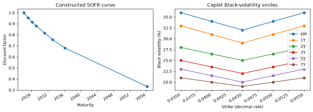
The SOFR curve specification selects deposit and OIS calibration quotes, with day-count and interpolation conventions for the constructed curve. The surface specification selects caplet Black-volatility quotes and their expiry and strike coordinates.

We reconstruct these configurations from the loaded dictionaries to make the conventions visible. The quote lists remain in the companion market data.

curve_spec = market.curves[0].to_dict()
curve_config = qs.CurveConfiguration.from_dict(curve_spec)
surface_spec = market.volatility_surfaces[0].to_dict()
surface_config = qs.VolatilitySurfaceConfiguration.from_dict(
    {
        **surface_spec,
        "market_index": qs.MarketIndex.SOFR,
        "volatility_type": qs.VolatilityType.Black,
        "smile_type": qs.SmileType.Strike,
    }
)
print(
    "Curve conventions:",
    {key: value for key, value in curve_spec.items() if key != "quotes"},
)
print(
    "Surface conventions:",
    {key: value for key, value in surface_spec.items() if key != "quotes"},
)
print(
    "Curve quotes:",
    len(curve_spec["quotes"]),
    "| Volatility quotes:",
    len(surface_spec["quotes"]),
)

Curve conventions: {'day_counter': 'Actual360', 'enable_extrapolation': True, 'interpolator': 'LogLinear', 'market_index': 'SOFR'}
Surface conventions: {'extrapolation_policy': 'Reject', 'market_index': 'SOFR', 'smile_type': 'Strike', 'volatility_type': 'Black'}
Curve quotes: 8 | Volatility quotes: 27

Observe nodes, forwards, and the smile

Query the constructed objects inside an active context. nodes() returns dated discount factors; pillars() returns labels used to trace risk back to inputs. A forward rate is inferred from discount factors over the requested interval under the selected compounding convention.

This surface’s smile coordinate is an absolute strike, so 0.045 means a 4.5% strike, not a delta or log-moneyness. Its values are decimal Black vols. The grid below stays within the supplied quote domain and includes an intermediate strike so the interpolation is visible.

expiries = ["6M", "1Y", "2Y", "3Y", "5Y", "7Y"]
strikes = [0.035, 0.040, 0.045, 0.050, 0.055]
context = qs.PricingContext(
    quotes=market.quotes,
    curves=[curve_config],
    csa_policy=market.csa_policy,
    volatility_surfaces=[surface_config],
)

with context:
    curve = context.curve(qs.MarketIndex.SOFR)
    surface = context.volatility_surface(qs.MarketIndex.SOFR)
    nodes = curve.nodes()
    pillars = curve.pillars()
    forward_rows = []
    for tenor in ["1Y", "2Y", "3Y", "5Y", "7Y"]:
        start_date = ref + tenor
        end_date = start_date + "1Y"
        forward_rate = curve.forward_rate(
            start_date, end_date, qs.Compounding.Simple, qs.Frequency.Annual
        )
        forward_rows.append(
            {
                "start": tenor,
                "discount_factor": curve.discount_factor(start_date),
                "one_year_forward": forward_rate,
            }
        )
    forwards = pd.DataFrame(forward_rows)

    smile = pd.DataFrame(index=pd.Index(strikes, name="strike"))
    for expiry in expiries:
        smile[expiry] = [surface.volatility(expiry, strike) for strike in strikes]
    print(surface.volatility_type, surface.smile_type)

forwards

Black Strike

	start	discount_factor	one_year_forward
0	1Y	0.953257	0.042106
1	2Y	0.914227	0.036951
2	3Y	0.881127	0.037741
3	5Y	0.817367	0.039061
4	7Y	0.756187	0.035225

fig, axes = plt.subplots(1, 2, figsize=(11, 4))
axes[0].plot(pd.to_datetime(nodes["date"]), nodes["discount_factor"], marker="o")
axes[0].set(title="Constructed SOFR curve", xlabel="Maturity", ylabel="Discount factor")
(smile * 100).plot(ax=axes[1], marker="o")
axes[1].set(
    title="Caplet Black-volatility smiles",
    xlabel="Strike (decimal rate)",
    ylabel="Black volatility (%)",
)
fig.autofmt_xdate()
plt.tight_layout()
plt.show()

Revaluation under changed inputs

A quote scenario rebuilds the curve or surface from changed observations. The rate shock below selects the deposit and OIS identifiers, while the volatility shock uses one caplet-family selector.

Targets match sets of underscore-separated identifier segments. SOFR alone would select both rate and volatility quotes here. Full caplet identifiers can also overlap when tenor and expiry share a token, so listing every volatility identifier could move some quotes more than once. We use the single CapletFloorlet_USD_SOFR target and verify its transformed quotes below. An absolute shock adds the supplied amount; a relative shock multiplies by 1 + value.

swap = qs.Swap(
    identifier="SWAP",
    start_date=ref,
    maturity_date=ref + "5Y",
    notional=1_000_000,
    fixed_rate=0.04,
    currency=qs.Currency.USD,
    market_index=qs.MarketIndex.SOFR,
)
caplet = qs.CapletFloorlet(
    identifier="CAPLET",
    fixing_date=ref + "2Y",
    start_accrual_date=ref + "2Y",
    end_accrual_date=ref + "2Y3M",
    payment_date=ref + "2Y3M",
    strike=0.045,
    currency=qs.Currency.USD,
    market_index=qs.MarketIndex.SOFR,
    payoff_type=qs.CapletFloorletType.Caplet,
)
swap_trade = qs.Trade(swap, ref)
caplet_trade = qs.Trade(caplet, ref, notional=1_000_000)
rate_up = [
    qs.Shock(target=label, value=0.001, shock_type=qs.ScenarioType.Absolute)
    for label in curve_spec["quotes"]
]
vol_up = [
    qs.Shock(
        target="CapletFloorlet_USD_SOFR",
        value=0.01,
        shock_type=qs.ScenarioType.Absolute,
    )
]


def observe_market(shocks):
    context = qs.PricingContext(
        quotes=market.quotes,
        curves=[curve_config],
        csa_policy=market.csa_policy,
        volatility_surfaces=[surface_config],
    )

    with context, qs.Scenario(shocks=shocks):
        return {
            "swap_pv_usd": context.evaluate(swap_trade).price,
            "caplet_pv_usd": context.evaluate(caplet_trade).price,
            "five_year_df": context.curve(qs.MarketIndex.SOFR).discount_factor(
                ref + "5Y"
            ),
            "two_year_vol": context.volatility_surface(qs.MarketIndex.SOFR).volatility(
                "2Y", 0.045
            ),
        }


comparison = pd.DataFrame(
    {
        "base": observe_market([]),
        "rates +10 bp": observe_market(rate_up),
        "vols +1 point": observe_market(vol_up),
    }
).T
comparison["swap_pnl_usd"] = (
    comparison["swap_pv_usd"] - comparison.loc["base", "swap_pv_usd"]
)
comparison["caplet_pnl_usd"] = (
    comparison["caplet_pv_usd"] - comparison.loc["base", "caplet_pv_usd"]
)
comparison

	swap_pv_usd	caplet_pv_usd	five_year_df	two_year_vol	swap_pnl_usd	caplet_pnl_usd
base	-1664.991324	571.899568	0.817367	0.25	0.000000	0.000000
rates +10 bp	-6081.828255	649.084288	0.813418	0.25	-4416.836932	77.184721
vols +1 point	-1664.991324	615.801139	0.817367	0.26	0.000000	43.901571

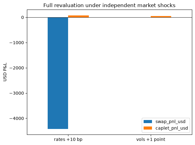
A higher rate market makes the agreed fixed coupon less attractive, reducing the receive-fixed swap’s PV. Its value stays unchanged under the separate volatility move. The caplet gains from higher Black volatility; its rate response combines changes in the forward and discount factor.

comparison[["swap_pnl_usd", "caplet_pnl_usd"]].iloc[1:].plot.bar(
    title="Full revaluation under independent market shocks", ylabel="USD P&L", rot=0
)
plt.axhline(0, color="black", linewidth=0.7)
plt.tight_layout()
plt.show()

Interpolation and scenario checks

At a quoted expiry, this surface interpolates linearly between adjacent strikes:

\[\sigma(K)=(1-w)\sigma(K_0)+w\sigma(K_1),\qquad w=\frac{K-K_0}{K_1-K_0}.\]

We check an intermediate strike against the two quoted volatilities, then verify that the volatility shock moves each intended quote once and leaves rate quotes unchanged. The resulting curve and surface queries confirm which market objects changed.

quotes = market.quotes.to_dataframe().set_index("identifier")["mid"]
low_label = "CapletFloorlet_USD_SOFR_3M_2Y_Absolute_0.035_Straddle_Black"
high_label = "CapletFloorlet_USD_SOFR_3M_2Y_Absolute_0.045_Straddle_Black"
interpolated_vol = (quotes.loc[low_label] + quotes.loc[high_label]) / 2
with context, qs.Scenario(shocks=vol_up):
    bumped_quotes = context.quotes.to_dataframe().set_index("identifier")["mid"]
quote_moves = bumped_quotes - quotes
print(f"Interpolated 2Y Black vol at 4% strike: {interpolated_vol:.2%}.")
print("Independent shocks leave the unrelated market object unchanged.")
comparison[["swap_pnl_usd", "caplet_pnl_usd", "five_year_df", "two_year_vol"]]

Interpolated 2Y Black vol at 4% strike: 26.50%.
Independent shocks leave the unrelated market object unchanged.

	swap_pnl_usd	caplet_pnl_usd	five_year_df	two_year_vol
base	0.000000	0.000000	0.817367	0.25
rates +10 bp	-4416.836932	77.184721	0.813418	0.25
vols +1 point	0.000000	43.901571	0.817367	0.26

The two scenario P&Ls show the swap’s rate exposure and the caplet’s joint rate and volatility dependence. The interpolation check also identifies the quantity being interpolated: Black volatility at a strike, with the configured expiry conventions.

The portfolio-risk study compares local quote derivatives with small full-revaluation bumps. For simulated rates or callable bonds, calibration adds another step by converting Black option prices into absolute short-rate model sigmas.